20.15 — Meta-analysis
Introduction
Meta-analysis is a type of systematic review (Greenhalgh 1997, Akobeng 2005), a statistical method used to combine the results from multiple independent studies that addressed the same topic. By combining studies, the goal is to calculate a pooled estimate as a measure of overall effectiveness of the treatment. The underlying logic is that multiple studies draw subjects from the same reference population, thus, combining data provides a more powerful test of the hypothesis.
Meta-analysis can increase the overall sample size, which improves the study’s ability to detect an effect if one exists. So, how to combine results from different studies ostensibly addressing the same hypothesis? Inevitably, some subjectivity will come into decisions about including or excluding studies — the goal is to identify quality studies, which may have conflicting conclusions and test whether a single conclusion of effectiveness is warranted based on a summary of evidence.
Meta-analysis is now a routine type of study, conducted in multiple disciplines, including biomedical field (eg, Cochrane Reviews, more than 15K since 1993, Anderson et al 2024), and environmental studies (eg, Resende et al 2021), and sports science (eg, Miyamoto-Mikami et al 2018).
In general, meta-analysis studies return the combined effect size –the single, pooled effect across all included studies — of an intervention and the heterogeneity among the studies — how consistent measured differences. Models may be fixed effects — that is, any observed differences among studies are due to chance or sampling error — or random effects — the true effect size varies from study to study and that these effects are drawn from a distribution.
The purpose of this page is to provide a basic overview and an introduction to the meta-analysis approach. We previously introduced the Cochran’s Q test aka heterogeneity  test in Chapter 9.4. The chi-square test test asks whether results from combined studies are consistent. After discussing inclusion criteria, we provide plotting techniques and additional statistical tests for heterogeneity of studies.
In Chapter 12.4, we introduced a simple meta-analysis combining ten separate one sample t-tests of the hypothesis that inbred mice and genetically diverse mouse strains do not differ for average lifespan. P-values were combined and we used Fisher’s method to evaluate the hypothesis.
Note 1: The most robust and recommended method for meta-analysis is to use effect sizes (eg, standardized mean differences, odds ratios, risk ratios) and their corresponding standard errors or confidence intervals (Nakagawa and Cuthill 2007). This approach avoids the limitations of arbitrary p-value thresholds and provides a more complete picture of the effect’s magnitude and precision.
Selection criteria
Any project, whether an observational study or an experiment, starts with a question that is modified into one or more testable hypothesis. We don’t collect the data then speculate about causes for perceived patterns that may appear. Rather, pattern recognition process can be used to generate hypotheses subject to future testing. Our example was about lifespan and genetic background and genetic diversity: Longevity refers to the capacity to live a long life whereas lifespan is the maximum amount of time an individual can live. We ask if genetic diversity increases longevity across a population; specific genetic background is linked to an individual’s predisposition to long life.
Given the importance such work has in clinical research, as you can imagine, there is plenty of advice and suggested guidelines for how to proceed. Of note, review systematic review Population, Intervention, Comparison, Outcome (PICO) guidelines (Schardt et al 2007). Additionally, see the Cochrane Handbook (2024).
With a clear hypothesis in hand, for both systematic review and meta-analysis, the study begins with a search of the published literature. Search results from the query “inbred mice strain lifespan,” in Pubmed returned about 1134 publications; replacing “longevity” for “lifespan,” returned 654 publications. We want primary literature, not reviews, so we add NOT (Review[Publication Type]) to the query: 1080 and 617, respectively. Further restricting the pool by restricting range to last ten years returned a manageable 197 and 116 results, respectively. We can begin selecting our data from the studies. We now have to decide whether all or only some meet our standards for consideration. Of course, this is not the same thing as looking at the results and selecting only the studies that confirm our thinking! Ideally, reporting of both positive (large effect size, small p-value) and negative (small effect size, large p-value) studies can — and should — be included. Our goal, combine the results of multiple independent studies on the same topic to reach a more powerful and reliable conclusion than a single study could provide.
Note 2: Publication bias concerns likely overestimates of effect size for meta-analysis, just as the tendency for reporting only “statistically significant” p-values (Ioannidis 2008).
Inclusion criteria are the requirements a study must meet to be considered for the review; exclusion criteria are the specific reasons a study is disqualified. Decisions about which studies to include consider demographics, intervention type, and study design. For example, the review may focus only on RCT studies. Likely, the review is focused on experimental work and so, excluding previous systematic reviews would be an example of an exclusion criteria. At the same time we need to be transparent about our approach; that includes defining a clear research question, establishing strict inclusion/exclusion criteria, conducting a comprehensive literature search across multiple databases, and performing a rigorous data extraction and quality assessment of included studies (Meline 2006, Paldam 2015, Cochrane Handbook). For our lifespan and genetic diversity example I found two studies that met my criteria: the studies needed multiple inbred strains or outbred strains and the raw data needed to be available. Two studies met this need: Yuan et al (2009) and Mullis et al (2025).
An imperfect example. To practice applying selection and exclusion criteria for a meta-analysis, I ran a PubMed search using the keywords botox migraine. I limited the results to clinical trials published within the past five years, which gave me 14 papers. I read the abstracts and decided to include studies only if they had a control group, focused on patients with chronic migraine, and reported an exact p-value instead of just saying “P < 0.05.” Table 1 shows what I found, including the PubMed link for each paper, whether it was included, the sample size, the p-value, and my comments on why any studies were excluded.
Table 1. Example data collection for meta-analysis, topic botox and treatment of chronic migraines.
| paper | Include | N | p-value | Why exclude? |
|---|---|---|---|---|
| https://pubmed.ncbi.nlm.nih.gov/37499085/ | No | review | ||
| https://pubmed.ncbi.nlm.nih.gov/38982666/ | Yes | 1384 | 0.01 | |
| https://pubmed.ncbi.nlm.nih.gov/37994890/ | No | 209 | 0.155 | no control group |
| https://pubmed.ncbi.nlm.nih.gov/41091731/ | No | 775 | > 0.05 | no CI, no exact p-value |
| https://pubmed.ncbi.nlm.nih.gov/34404257/ | No | 32 | 0.03 | within subjects design, no control group |
| https://pubmed.ncbi.nlm.nih.gov/37315247/ | Yes | 209 | 0.365 | |
| https://pubmed.ncbi.nlm.nih.gov/33722518/ | No | 60 | < 0.001 | within subjects design, no control group, no exact p-value |
| https://pubmed.ncbi.nlm.nih.gov/36189948/ | No | 0.092 | no sample size, no control | |
| https://pubmed.ncbi.nlm.nih.gov/36189948/ | No | 0.174 | no sample size, no control | |
| https://pubmed.ncbi.nlm.nih.gov/35166150/ | No | method paper | ||
| https://pubmed.ncbi.nlm.nih.gov/33106278/ | Yes | 15 | 0.038 | |
| https://pubmed.ncbi.nlm.nih.gov/37235358/ | No | 139 | < 0.0001 | no CI, no exact p-value |
| https://pubmed.ncbi.nlm.nih.gov/35064733/ | No | overuse, not migraine | ||
| https://pubmed.ncbi.nlm.nih.gov/33241323/ | No | PTH, not migraine | ||
| https://pubmed.ncbi.nlm.nih.gov/32873093/ | No | no control group |
That leaves only three papers, not enough for a meta-analysis. By changing years from five to ten, 40 papers were available to search. By removing all time restrictions, 109 papers were returned since year 2000. Medical use of botox dates to the 1970s (Scott 2023).
R packages
metafor package: provides extensive functions for calculating various effect sizes, fitting different statistical models (e.g., fixed- and random-effects, mixed-effects), conducting meta-regression, and generating numerous meta-analytical plots.
See also metaforGUI package which provides a Graphical User Interface (GUI) for the R metafor Package.
meta package: provides user-friendly and comprehensive collection of functions for conducting standard meta-analyses.
Much has been written about how to conduct meta-analysis and caveat emptor — readers should be on notice that I present here just a fraction of the “how to” and pitfalls of meta-analysis. Interested readers should see Doing meta-analysis with R: A hands-on guide by M. Harrer et al (2021).
I2 or I-squared test
In a meta-analysis, the I-squared test  quantifies the percentage of total variation in a set of study results that is due to differences between studies rather than random sampling error (chance). An of 0% means all variation is due to chance, while a higher percentage indicates that differences between studies are a significant source of variation. As a reminder, the test returns a p-value that can be used to interpret whether that heterogeneity is statistically significant. We run our life span of inbred and genetically diverse outbred mouse strains example in Chapter 12.4; the p-value was small — we used Fisher’s method p-value combination approach to test the main hypothesis.
Here, we calculate ; we first need the effect size; Cohen’s d (Chapter 11.4) will do.
Table 1. Updated Table 1 from Chapter 12.4.
| Strain | n | mean | sd | cohen’s d | V(d) |
| 129S1/SvImJ | 32 | 787.4 | 159.16 | 0.045 | 0.191 |
| A/J | 32 | 630.7 | 130.20 | 1.26 | 0.04 |
| BALB/cByJ | 32 | 734.4 | 154.43 | 0.389 | 0.0368 |
| BUB/BnJ | 24 | 611.3 | 218.34 | 0.839 | 0.0485 |
| C3H/HeJ | 29 | 724.1 | 131.48 | 0.536 | 0.0403 |
| C57BL/6J | 29 | 855.7 | 185.34 | 0.330 | 0.0399 |
| CBA/J | 30 | 622.9 | 181.95 | 0.943 | 0.0405 |
| FVB/NJ | 26 | 750.3 | 230.11 | 0.192 | 0.0438 |
| P/J | 32 | 676.0 | 178.82 | 0.663 | 0.0374 |
| SWR/J | 31 | 831.9 | 181.31 | 0.206 | 0.0376 |
The effect size ranged from practically no difference (Cohen’s d of 4.5%) to substantial effect on average lifespan of inbred vs outbred strains (Cohen’s d of 126%). The simple average of the Cohen’s d values was 0.541; a weighted average accounting for differences in variance needs to be applied. Regardless, the statistic we want is the coefficient from meta-regression, which indicates how a change in that predictor relates to the effect size.
Note 3: The greatest effect size — difference in average lifespan — was reported for the A/J strain — this strain is primarily used in cancer research because of its susceptibility to cancers. The smallest effect size was for the 129S1/SvImJ strain, which is used for creating genetically modified mice.
With effect size calculated, we proceed to get . We use rma() from metafor package. This function performs several tests: a fixed-effects model and therefore we test a model where we assume all studies found the exact same effect, a random-effects model where the assumption is that effects are similar but vary across studies, plus a mixed-effects model uses a combination of both, and finally, a meta-regression. The meta-regression uses the data from those studies to try and explain why the results differ.
R code
library(metafor)
strains <- 1:10
my_effsize <- c(0.0446092, 1.258065, 0.3891731, 0.8390583,
0.5354427, 0.3302039, 0.9431162, 0.192082, 0.6626776, 0.2062765)
my_sample <- c(32, 32, 32, 24, 29, 29, 30, 26, 32, 31)
my_varC <- (my_effsize^2)/(2*my_sample)
myData <- data.frame(strains, my_effsize, my_sample, my_varC)
rma(yi = my_effsize, vi = my_varC, data = myData)
R output
Random-Effects Model (k = 10; tau^2 estimator: REML)

tau^2 (estimated amount of total heterogeneity): 0.1299 (SE = 0.0643)
tau (square root of estimated tau^2 value): 0.3604
I^2 (total heterogeneity / total variability): 99.15%
H^2 (total variability / sampling variability): 117.11

Test for Heterogeneity:
Q(df = 9) = 390.9415, p-val < .0001

Model Results:

estimate     se   zval   pval  ci.lb  ci.ub
  0.5208 0.1169 4.4558 <.0001 0.2917 0.7499 ***
---
Signif. codes: 0 ‘***’ 0.001 ‘**’ 0.01 ‘*’ 0.05 ‘.’ 0.1 ‘ ’ 1
Interpretation.
With an of 99%, which suggests a very high degree of heterogeneity among the comparison between the DO strain and the ten inbred strains for life span. As before, the heterogeneity or Q test was highly statistically significant, suggests that the observed variability is larger than what would be expected due to chance alone. Thus, all of the variability in the observed effects comes from between-strain differences, not random chance — it also justifies use of a random effects model, not a fixed model. Strain A/J, with the greatest difference in lifespan compared to the DO strain, is recognized for its susceptibility to carcinogenic tumors
From the meta regression, the coefficient was 0.52 — inbred strain membership was associated with change in the size of the effect. We conclude that in general, the genetically inbred strains differ substantially for average lifespan compared to the genetically variable DO strain: The true average effect was somewhere between 0.2917 and 0.7499.
Our results conform to our expectations — longevity is likely affected by a combination of effects from many genes along with an individual’s genetic background and interaction with the environment, cf discussion in Mullis et al (2025).
Forest plot of effect size.
A forest plot visually summarizes results from multiple studies, showing each study’s effect size (eg, odds ratio, mean difference, Cohen’s d) and variance or confidence interval as squares and lines, plus the overall pooled estimate (diamond). It helps quickly assess study consistency (heterogeneity), see individual study contributions, and determine if the combined evidence points to a significant overall effect.
For example, our inbred strains vs the outbred DO strain for lifespan shows a clear, overall effect (Fig 1). The diverse genetic strain lifespan is significantly greater than the majority of inbred strains, and the combined effect is about 0.5.
R code
library(metafor)
myData <- data.frame(
Strains = paste("Strains", c("129S1/SvImJ", "A/J", "BALB/cByJ", "BUB/BnJ",
"C3H/HeJ", "C57BL/6J", "CBA/J", "FVB/NJ", "P/J", "SWR/J")),
cohenD = c(0.045, 1.26, 0.389, 0.839, 0.536, 0.33, 0.943, 0.192, 0.663, 0.206),
cohenV = c(0.1910, 0.0400, 0.0368, 0.0485, 0.0403, 0.0399, 0.0405, 0.0438, 0.0374, 0.0376)
)

res2 <- rma(cohenD, cohenV, data = myData, method="REML")
# str(res2)

forest(res2,
slab = myData$Strains,
xlab = "Cohen's d")
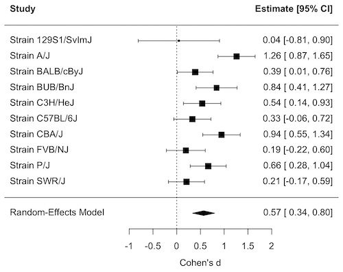
Figure 1. Forest plot, Cohen’s effect size lifespan differences among inbred strains of mice compared to outbred strain.
Questions
1. What’s the difference between a literature review and a systematic review?
2. For which kinds of research goals would a meta-analysis be more appropriate than a systematic review?
Quiz Chapter 20.15
Meta-analysis
References and suggested readings
Akobeng, A. K. (2005). Understanding systematic reviews and meta-analysis. Arch Dis Child, 90:845-848.
Andersen, M. Z., Zeinert, P., Rosenberg, J., & Fonnes, S. (2024). Comparative analysis of Cochrane and non-Cochrane reviews over three decades. Systematic Reviews, 13, 120.
Cochrane reviews, Cochrane Library. (2025). https://www.cochranelibrary.com/
Greenhalgh, T. (1997). How to read a paper: Papers that summarise other papers (systematic reviews and meta-analyses). BMJ, 315(7109), 672–675.
Gurevitch, J., Koricheva, J., Nakagawa, S., & Stewart, G. (2018). Meta-analysis and the science of research synthesis. Nature, 555(7695), 175–182.
Hansen, C., Steinmetz, H., & Block, J. (2022). How to conduct a meta-analysis in eight steps: A practical guide. Management Review Quarterly, 72(1), 1–19.
Harrer, M., Cuijpers, P., Furukawa, T.A., & Ebert, D.D. (2021). Doing Meta-Analysis with R: A Hands-On Guide. Boca Raton, FL and London: Chapman & Hall/CRC Press. Link to website.
Ioannidis, J. P. A. (2008). Why Most Discovered True Associations Are Inflated. Epidemiology, 19(5), 640.
Higgins JPT, Thomas J, Chandler J, Cumpston M, Li T, Page MJ, Welch VA (editors). Cochrane Handbook for Systematic Reviews of Interventions version 6.5 (updated August 2024). Cochrane, 2024. Available from www.cochrane.org/handbook.
Meline, T. (2006). Selecting studies for systemic review: Inclusion and exclusion criteria. Contemporary Issues in Communication Science and Disorders, 33(Spring), 21–27.
Miyamoto-Mikami, E., Zempo, H., Fuku, N., Kikuchi, N., Miyachi, M., & Murakami, H. (2018). Heritability estimates of endurance-related phenotypes: A systematic review and meta-analysis. Scandinavian Journal of Medicine & Science in Sports, 28(3), 834–845.
Mullis, M. N., Wright, K. M., Raj, A., Gatti, D. M., Reifsnyder, P. C., Flurkey, K., Archer, J. R., Robinson, L., Di Francesco, A., Svenson, K. L., Korstanje, R., Harrison, D. E., Ruby, J. G., & Churchill, G. A. (2025). Analysis of lifespan across diversity outbred mouse studies identifies multiple longevity-associated loci. Genetics, 230(4), iyaf081.
Nakagawa, S., & Cuthill, I. C. (2007). Effect size, confidence interval and statistical significance: A practical guide for biologists. Biological Reviews, 82(4), 591–605.
Paldam, M. (2015). Meta-analysis in a nutshell: Techniques and general findings. Economics, 9(1), 20150011.
Resende, P. S., Viana-Junior, A. B., Young, R. J., & Azevedo, C. S. (2021). What is better for animal conservation translocation programmes: Soft- or hard-release? A phylogenetic meta-analytical approach. Journal of Applied Ecology, 58(6), 1122–1132.
Schardt, C., Adams, M. B., Owens, T., Keitz, S., & Fontelo, P. (2007). Utilization of the PICO framework to improve searching PubMed for clinical questions. BMC Medical Informatics and Decision Making, 7, 16.
Scott, A. B., Honeychurch, D., & Brin, M. F. (2023). Early development history of Botox (onabotulinumtoxinA). Medicine, 102(Suppl), e32371.
van Aert, R. C. M., Wicherts, J. M., & van Assen, M. A. L. M. (2016). Conducting Meta-Analyses Based on p Values. Perspectives on Psychological Science, 11(5), 713–729.
Yuan, R., Tsaih, S.-W., Petkova, S. B., de Evsikova, C. M., Xing, S., Marion, M. A., Bogue, M. A., Mills, K. D., Peters, L. L., Bult, C. J., Rosen, C. J., Sundberg, J. P., Harrison, D. E., Churchill, G. A., & Paigen, B. (2009). Aging in inbred strains of mice: Study design and interim report on median lifespans and circulating IGF1 levels. Aging Cell, 8(3), 277–287.
Chapter 20 contents
- Additional topics
- Area under the curve
- Peak detection
- Baseline correction
- Surveys
- Time series
- Dimensional analysis
- Estimating population size
- Diversity indexes
- Survival analysis
- Growth equations and dose response calculations
- Plot a Newick tree
- Phylogenetically independent contrasts
- How to get the distances from a distance tree
- Binary classification
- Meta-analysis
18.4 – Generalized Linear Squares
Introduction
With access to powerful computers and better algorithms, we can move past the classical ANOVA and ordinary least squares approaches to linear models. We have discussed general linear models, but here we introduce generalized linear models, GLM, not to be confused with the general linear model introduced in Chapter 12.7. The GLM is an extension or generalization of the general linear model, which assumes the outcome variable comes from a normal distribution. The chief advantage of GLM approaches is that we no longer need to make assumptions about the error variance, for example — now, we can specify the model structure and account for correlated errors and other deviations. What follows on this page is just a brief foray into GLS, generalized least squares; GLS is a method of parameter estimation. For more — and better! discussion, see Zuur et al (2009) and Dobson and Barnett (2018).
Model variances
In Generalized Least Squares (GLS) models, varPower and varExp are used to model heterogeneous variances (heteroscedasticity) that change as a function of a continuous covariate. varPower models the variance as proportional to a power of the absolute value of a covariate; this is useful when the spread of residuals increases or decreases in a power-law fashion with a predictor. In contrast, varExp models the variance as an exponential function of a covariate; this structure may be better when the variance increases rapidly.
Data from Corn and Hiesey (1973) ohia.RData
head(ohia)
   Site  Height   Width
1   M-1 12.5567 19.1264
2   M-1 13.2019 13.1547
3   M-1  8.0699 16.0320
4   M-1  6.0952 22.8586
5   M-1 11.3879 11.0105
6   M-1 12.2242 21.8102
A reminder, what we did before. Note that # ignore the variance issue
AnovaModel.1 <- aov(Height ~ Site, data = ohia); summary(AnovaModel.1)
           Df Sum Sq Mean Sq F value      Pr(>F)
Site        2   4070  2034.8   22.63 0.000000131 ***
Residuals  47   4227    89.9
---
Signif. codes: 0 '***' 0.001 '**' 0.01 '*' 0.05 '.' 0.1 ' ' 1
Alternatively, use gls(). Default fits by restricted maximum likelihood, REML. That is, it’s the likelihood of linear combinations of the original data. This first pass, we ignore issues about error variances, in other words, an approach similar to the ANOVA we did before.
model.aov.1 <- gls(Height ~ Site, data = ohia)

Generalized least squares fit by REML
Model: Height ~ Site
Data: ohia
     AIC      BIC    logLik
361.1312 368.5318 -176.5656

Coefficients:
                Value Std.Error  t-value p-value
(Intercept) 15.313745  2.120550 7.221591  0.0000
Site[T.M-2] 19.261000  2.998911 6.422666  0.0000
Site[T.M-3]  2.924215  3.672900 0.796160  0.4299

Correlation:
            (Intr) S[T.M-2
Site[T.M-2] -0.707
Site[T.M-3] -0.577   0.408

Standardized residuals:
       Min         Q1        Med        Q3       Max
-1.9832938 -0.5020880 -0.1850871 0.5017636 3.0850635

Residual standard error: 9.483388
Degrees of freedom: 50 total; 47 residual
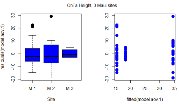
Figure 1. Box plot of residuals from GLS model by elevation site predictors (left) and scatterplot of residuals by fitted values from GLS model (right).
Inspection of Figure 1 suggests residuals not equal — note restricted range of intervals for the M-2 site.
R code for the plot in Figure 1
par(mfrow = c(1, 2))
plot(residuals(model.aov.1) ~ Site, pch=19, cex=1.5,col="blue", data = ohia)
plot(residuals(model.aov.1) ~ fitted(model.aov.1), pch=19, cex=1.5, col="blue", ylab="", data=ohia)
mtext("ANOVA Ohi`a Height, 3 Maui sites ", side = 3, line = -3, outer = TRUE)
So, our conventional approach would be to investigate the assumption of equal error variances.
# test equal variances, Height
leveneTest(Height ~ Site, data=ohia, center="median")
Levene's Test for Homogeneity of Variance (center = "median")
      Df F value  Pr(>F)
group  2  2.1663  0.1259
      47
We would conclude no significant departures from equal variances by Levene test. Consider Bartlett’s test.
bartlett.test(Height ~ Site, data=ohia)

Bartlett test of homogeneity of variances

data:  Height by Site
Bartlett's K-squared = 10.373, df = 2, p-value = 0.005592
In conclusion, there’s some evidence of unequal variances. We revisit the Generalized Linear Model approach, this time accounting for unequal variances as part of model
model.aov.3 <- gls(Height ~ Site, data = ohia, weights = varIdent(form = ~1|Site)); summary(model.aov.3)
Generalized least squares fit by REML
Model: Height ~ Site
Data: ohia
    AIC      BIC    logLik
354.421 365.5219 -171.2105
varIdent permits variances for each group to vary.
Results from R continue below.
Variance function:
 Structure: Different standard deviations per stratum
 Formula: ~1 | Site
 Parameter estimates:
      M-1       M-2       M-3
1.0000000 1.0396880 0.3471771
We see here that comparisons were carried out versus M-1 site.
Coefficients:
                Value Std.Error  t-value p-value
(Intercept) 15.313745  2.280931 6.713812  0.0000
Site[T.M-2] 19.261000  3.290358 5.853770  0.0000
Site[T.M-3]  2.924215  2.541027 1.150800  0.2556
Marginal differences between M-1 and M-2 for height were significantly different, but not between M-1 and M-3 site.
Correlation:
            (Intr) S[T.M-2
Site[T.M-2] -0.693
Site[T.M-3] -0.898   0.622

Standardized residuals:
       Min         Q1        Med        Q3       Max
-1.7734556 -0.6909962 -0.2108834 0.5801370 2.7586550

Residual standard error: 10.20064
Degrees of freedom: 50 total; 47 residual
# Test the models
> anova(model.aov.1, model.aov.3)
            Model df      AIC      BIC    logLik   Test  L.Ratio p-value
model.aov.1     1  4 361.1312 368.5318 -176.5656
model.aov.3     2  6 354.4210 365.5219 -171.2105 1 vs 2  10.7102 0.0047
Although additional degrees of freedom are required, note that this model (model.aov.3) has higher (better!) log likelihood (-171.21) than model.aov.1, the gls model lacking a fit for different variances (-176.57). Introduce a test of the hypothesis that the two models are equal by comparing the log (natural) likelihoods, the log likelihood ratio test, LRT.
![\begin{align*} LRT=-2\cdot ln\left ( \frac{LL\ model \1}{LL \ model \2} \right ) = -2\cdot ln \left [ \left (LL\ model \1 \right ) - \left (LL \ model \2 \right ) \right ] \end{align*}](https://biostatistics.letgen.org/wp-content/ql-cache/quicklatex.com-a5d504cb562cdafece753076d69c0ed8_l3.png "Rendered by QuickLaTeX.com")
The LRT follows a chi-square distribution (per Wilk’s theorem). If there was no advantage to fitting for unequal variances, then the model fit would not be improved and p-value of the LRT would not be less than 5%.
Conclusion
You can see why this approach, even for the rather simple example in this case, modeling versus separate test of assumptions would be the preferred way to go. We get a better fitting model, and, we have employed proper statistical practice (Dobson and Barnett 2018).
Another example, same data set. R code follows.
# ignore variances, Width
model.aov.2 <- gls(Width ~ Site, data = ohia); summary(model.aov.2)
Figure 2.
par(mfrow = c(1, 2))
plot(residuals(model.aov.2) ~ Site, pch=19, cex=1.5,col="blue", data = ohia)
plot(residuals(model.aov.2) ~ fitted(model.aov.2), pch=19, cex=1.5, col="blue", ylab="", data=ohia)
mtext("ANOVA Ohi`a Width 3 Maui sites ", side = 3, line = -3, outer = TRUE)

# test equal variances, Width
Tapply(Width ~ Site, var, na.action=na.omit, data=ohia) # variances by group
leveneTest(Width ~ Site, data=ohia, center="median")
Tapply(Width ~ Site, var, na.action=na.omit, data=ohia) # variances by group
bartlett.test(Width ~ Site, data=ohia)

# model the variances, Height

library(nlme)
model.aov.3 <- gls(Height ~ Site, data = ohia, weights = varIdent(form = ~1|Site)); summary(model.aov.3)
par(mfrow = c(1, 2))
plot(residuals(model.aov.3) ~ Site, pch=19, cex=1.5,col="red", data = ohia)
plot(residuals(model.aov.3) ~ fitted(model.aov.3), pch=19, cex=1.5, col="red", ylab="", data=ohia)
mtext("GLS Ohi`a Height 3 Maui sites ", side = 3, line = -3, outer = TRUE)

# Test the models
anova(model.aov.1, model.aov.3)

# model the variances, Width
model.aov.4 <- gls(Width ~ Site, data = ohia, weights = varIdent(form = ~1|Site)); summary(model.aov.4)
par(mfrow = c(1, 2))
plot(residuals(model.aov.4) ~ Site, pch=19, cex=1.5,col="red", data = ohia)
plot(residuals(model.aov.4) ~ fitted(model.aov.4), pch=19, cex=1.5, col="red", ylab="", data=ohia)
mtext("GLS Ohi`a Width 3 Maui sites ", side = 3, line = -3, outer = TRUE)

# Test the models
anova(model.aov.2, model.aov.4)
Interpretation
ccc
Model correlated residuals
When data points are not truly independent — repeated measurements on the same individual, or values taken along a spatial or temporal sequence — the residuals may show correlation. Generalized Least Squares (GLS) lets us model this correlation directly instead of pretending it isn’t there, as we might do in a multiple linear regression model. Ignoring correlated residuals may lead to underestimated standard errors and overconfident p-values. By specifying a correlation structure (such as autoregressive for time series, compound symmetry for repeated measures, or spatial correlation functions for location-based data), GLS adjusts the weighting of observations so that the model “knows” some points carry redundant information. The result is a more realistic fit, better inference, and parameter estimates that reflect how the data were actually generated.
Note 1: Time series analysis and the ARIMA and ARMA models are presented in Chapter 20.5.
We use the gls() function from the nlme package to model correlated residuals. The following is example code
# Load the nlme package
library(nlme)

# Create some example data with correlated residuals within groups
# (e.g., repeated measurements on different individuals)
set.seed(123)
n_subjects <- 10
n_obs_per_subject <- 5
data <- data.frame(
  Subject = factor(rep(1:n_subjects, each = n_obs_per_subject)),
  Time = rep(1:n_obs_per_subject, n_subjects),
  X = rnorm(n_subjects * n_obs_per_subject)
)
# Generate correlated errors within each subject
data$Y <- unlist(lapply(1:n_subjects, function(s) {
  errors <- arima.sim(model = list(ar = 0.7), n = n_obs_per_subject)
  10 + 2 * data$X[data$Subject == s] + errors
}))

# Fit a GLS model with an AR(1) correlation structure within each subject
# The 'correlation' argument specifies the correlation structure.
# corAR1() defines an AR(1) process.
# form = ~ 1 | Subject indicates that the AR(1) correlation applies within each 'Subject' group.
model_gls_ar1 <- gls(Y ~ X, data = data, correlation = corAR1(form = ~ 1 | Subject))
corAR1(form = ~ 1 | Subject) specifies an Autoregressive of order 1 (AR(1)) correlation structure, where the correlation is applied independently within each Subject group. The form = ~ 1 | Subject indicates that the correlation structure applies to observations within the same Subject group.
# Summarize the model results
summary(model_gls_ar1)
R output
> summary(model_gls_ar1)
Generalized least squares fit by REML
Model: Y ~ X
Data: data
AIC BIC logLik
148.7635 156.2483 -70.38176

Correlation Structure: AR(1)
Formula: ~1 | Subject
Parameter estimate(s):
Phi
0.2237348

Coefficients:
Value Std.Error t-value p-value
(Intercept) 10.294866 0.1668865 61.68782 0
X 2.155633 0.1478797 14.57693 0

Correlation:
(Intr)
X -0.034

Standardized residuals:
Min Q1 Med Q3 Max
-1.68711443 -0.85652175 0.02428734 0.59964691 2.38281397

Residual standard error: 0.9919801
Degrees of freedom: 50 total; 48 residual
Interpretation
The GLS model shows a strong positive relationship between X and Y: for every 1-unit increase in X, Y increases by about 2.16 units, on average, and this effect is highly statistically significant. The intercept (≈10.3) represents the expected value of Y when X is zero. Using a Generalized Least Squares approach improved the analysis because the data showed signs of correlated residuals—the AR(1) parameter (φ ≈ 0.22) indicates that measurements taken closer together within the same subject are moderately correlated. A standard linear model would incorrectly assume independence, which can make standard errors too small. By modeling the correlation directly, GLS produced more reliable standard errors and p-values, giving us greater confidence that the relationship between X and Y is real and not an artifact of ignored within-subject correlation.
Additional residual models
corCompSymm (compound symmetry) and corARMA (autoregressive moving average) are also provided as alternatives, demonstrating the flexibility of the nlme package for handling various correlation structures. Compound symmetry is a covariance structure that assumes all variances are equal and all covariances between any pair of measurements are equal. This means it assumes the correlation between any two repeated measurements within a subject is the same, regardless of how far apart they are in time or order. Autoregressive moving average is used for analyzing non-Gaussian time series data. Instead of fitting a standard ARMA to normally distributed data, GLARMA models handle data like counts or binary outcomes by modeling the conditional mean of the response, which belongs to a distribution from the exponential family (like Poisson or binomial), and using an ARMA structure for the linear predictor.
# Specify other correlation structures, eg, a compound symmetry correlation
model_gls_cs <- gls(Y ~ X, data = data, correlation = corCompSymm(form = ~ 1 | Subject))
summary(model_gls_cs)
R output
summary(model_gls_cs)
Generalized least squares fit by REML
  Model: Y ~ X
  Data: data
       AIC      BIC    logLik
  150.1495 157.6343 -71.07475

Correlation Structure: Compound symmetry
 Formula: ~1 | Subject
 Parameter estimate(s):
     Rho
0.100498

Coefficients:
                Value Std.Error  t-value p-value
(Intercept) 10.311332 0.1665215 61.92194       0
X            2.190527 0.1490535 14.69624       0

 Correlation:
  (Intr)
X -0.031

Standardized residuals:
         Min           Q1          Med           Q3          Max
-1.702766092 -0.878339355 -0.006044474  0.599317975  2.369540693

Residual standard error: 0.9939772
Degrees of freedom: 50 total; 48 residual
Interpretation
The GLS model again finds a clear positive association between X and Y: for each 1-unit increase in X, Y increases by about 2.19 units, and this effect is highly significant. The intercept (≈10.31) represents the expected value of Y when X is zero. In this version of the analysis, we used a compound symmetry (CS) correlation structure, which assumes that all observations within the same subject share the same correlation. The estimated within-subject correlation is modest (ρ ≈ 0.10), meaning repeated measurements on the same subject tend to be slightly more similar than measurements from different subjects.
Using GLS with CS has advantages when the repeated measures do not show a strong pattern of decay over time or order—unlike an AR(1) structure, which assumes that closer measurements are more correlated than farther ones. If the study design or exploratory plots suggest that all within-subject observations are roughly equally related, the CS structure is simpler, easier to interpret, and avoids imposing unnecessary assumptions. As a result, the model provides more accurate standard errors and p-values than an ordinary linear model while using an appropriate correlation pattern for the data.
Autocorrelation is expected in time series.
Time series data is a common source of correlated residuals because observations are sequential and related through time. Time series are basically repeated measures designs. When a standard regression model is applied to time-series data, the residuals would violate the assumption of independence and the model would fail to capture the temporal patterns.
Autoregressive Moving Average (ARMA) model is combined with Generalized Linear Models (GLMs) to handle non-Gaussian time series data. Instead of fitting a standard ARMA to normally distributed data, GLARMA models handle data like counts or binary outcomes by modeling the conditional mean of the response, which belongs to a distribution from the exponential family (like Poisson or binomial), and using an ARMA structure for the linear predictor.
# Or an autoregressive moving average (ARMA) structure:
# Note: corARMA takes additional arguments for p (AR order) and q (MA order)
model_gls_arma <- gls(Y ~ X, data = data, correlation = corARMA(p = 1, q = 1, form = ~ 1 | Subject))
summary(model_gls_arma)
R output
summary(model_gls_arma)
Generalized least squares fit by REML
  Model: Y ~ X
  Data: data
       AIC      BIC    logLik
  149.7441 159.1001 -69.87205

Correlation Structure: ARMA(1,1)
 Formula: ~1 | Subject
 Parameter estimate(s):
      Phi1     Theta1
-0.4316167  0.7078838

Coefficients:
                Value Std.Error  t-value p-value
(Intercept) 10.284066 0.1555666 66.10715       0
X            2.177237 0.1472516 14.78583       0

 Correlation:
  (Intr)
X -0.016

Standardized residuals:
        Min          Q1         Med          Q3         Max
-1.68468178 -0.86326393  0.03143835  0.62391661  2.40860526

Residual standard error: 0.9879063
Degrees of freedom: 50 total; 48 residual
Interpretation
We find again a strong, statistically significant relationship between X and Y: each 1-unit increase in X is associated with an increase of about 2.18 units in Y. The intercept (≈10.28) gives the expected value of Y when X is zero. In this model, we used an ARMA(1,1) correlation structure, which is more flexible than either the AR(1) or compound-symmetry forms. The ARMA parameters (φ₁ ≈ –0.43 and θ₁ ≈ 0.71) indicate that the residual correlation is not a simple “decay with lag” pattern (as in AR(1)) nor a uniform correlation across all observations (as in CS), but instead combines short-range autocorrelation with a moving-average component that can capture abrupt, short-term shocks or adjustments in the data.
Using GLS with an ARMA structure is advantageous when exploratory plots or diagnostics suggest complex within-subject dependence that neither AR(1) nor CS captures well. The ARMA model can better represent both smooth serial correlation and rapid error fluctuations, leading to more accurate standard errors, improved model fit (reflected here in a slightly lower AIC), and more trustworthy inference about the effect of X. Even though the estimated effect of X remains similar across all three models, the ARMA structure helps ensure that the uncertainty around that effect is appropriately estimated for this particular pattern of residual dependence.
Questions
1. Write up three learning outcomes for this page. Hint: Point your favorite generative AI to this page and ask for help.
Quiz Chapter 18.4
Generalized Linear Squares
Chapter 18 contents
20.14 – Binary classification
draft
Introduction
For much of this textbook we emphasized the search for causal explanations — applied (bio)statistics. Machine learning refers to any system used that churns data into predictions, while not necessarily explaining how the collection of predictors effect the outcome (Li and Tong 2022).
Classification in science is the act of grouping observations based on common features. In data science, classification procedures are used to predict which category a data point belongs to by finding the lines or planes — the decision boundary — that best divide the different classes.
Prediction or decision – use data to build or “train” a model that is then used to make future predictions or decisions given new data. Technically, prediction and decision are different concepts — prediction refers to what might happen given new information while decision is about what we may do given new information. We discussed prediction as a goal of regression models in some detail in Chapter 17 and Chapter 18.
Linear discriminant analysis (LDA) is a well known classification algorithm, whose roots trace back to R.A. Fisher. Linear discriminant analysis finds a linear combination of features that characterizes or separates two or more classes of objects or events. It builds on the idea of multiple linear regression: for multiple linear regression we predict a continuous outcome variable from a set of predictor variables; for discriminant analysis, we predict discrete outcomes, two or more mutually exclusive groups, from a set of predictor variables.
Logistic regression (LR) is another common classification algorithm. We previously introduced LR as a statistical method for modeling the dependence of a binomial outcome variable on one or more categorical or continuous predictor variables (see Chapter 18.3 – Logistic regression). LR shares many features with linear discriminant analysis, but while LDA models the distribution of the data and assumes normality for the predictor variables, LR directly models the probability of the outcome, making fewer assumptions about the distribution of the data. LDA returns a discriminant function, a linear combination of the features, while LR returns a probability between 0 and 1 via the logistic function, estimating the probability of the data point belonging to a specific class.
Both LDA and LR return single decision models — not the same classification model, of course. The downside for use of a single model to predict based on new data is that the assumptions used to build the model may not hold for the new data. Enter learning methods like random forest. Random forest is an example of supervised learning methods — it combines the predictions of multiple models to get a better result than any single model could achieve alone. The idea is that a “forest” of multiple decision trees are generated, trained on different subsets of data, which then contribute towards a classification choice based on the consensus of those many decision trees. By “training the model” in machine learning we imply a process by which we help an algorithm to recognize patterns in data to make predictions on new, unseen data. Model parameters are learned from the data during training, hyperparameters are settings that control the model training process.
Note 1: Supervised learning implies we use “labeled” data, where we already know to which group outcomes belong. Unsupervised learning uses unlabeled data to find hidden patterns or structures within the data.
R packages
caret — a “comprehensive package” for training and tuning predictive models. “Tuning” refers to optimizing the performance of a model by adjusting its hyperparameters.
ranger — for building random forest model of classification and regression models.
Questions
pending
Quiz
pending
References and suggested readings
Blei, D. M., & Smyth, P. (2017). Science and data science. Proceedings of the National Academy of Sciences, 114(33), 8689–8692.
Boehmke, B., & Greenwell, B. N. (2019). Hands-On Machine Learning with R. Chapman and Hall/CRC. https://bradleyboehmke.github.io/HOML/
Bzdok, D., Altman, N., & Krzywinski, M. (2018). Statistics versus machine learning. Nature Methods, 15(4), 233–234.
Hastie, T., Tibshirani, R., & Friedman, J. (2009). The Elements of Statistical Learning: Data Mining, Inference, and Prediction (2nd ed.). Springer.
Li, J. J., & Tong, X. (2020). Statistical hypothesis testing versus machine learning binary classification: Distinctions and guidelines. Patterns, 1(7).
Lin, X., Cai, T., Donoho, D., Fu, H., Ke, T., Jin, J., Meng, X.-L., Qu, A., Shi, C., Song, P., Sun, Q., Wang, W., Wu, H., Yu, B., Zhang, H., Zheng, T., Zhou, H., Zhou, J., Zhu, H., & Zhu, J. (2025). Statistics and AI: A Fireside Conversation. Harvard Data Science Review, 7(2).
Chapter 20 contents
- Additional topics
- Area under the curve
- Peak detection
- Baseline correction
- Surveys
- Time series
- Dimensional analysis
- Estimating population size
- Diversity indexes
- Survival analysis
- Growth equations and dose response calculations
- Plot a Newick tree
- Phylogenetically independent contrasts
- How to get the distances from a distance tree
- Binary classification
- Meta-analysis
19.3 — Monte Carlo methods
edits: — under construction —
Introduction
Statistical method that employ Monte Carlo methods use repeated random sampling to estimate properties of a frequency distribution. These distributions may be well-known, e.g., gamma-distribution, normal distribution, or t-distribution, or . The simulation is based on generation of a set of random numbers on the open interval (0,1) — the set of real numbers between zero and one (all numbers greater than 0 and less than 1).
If the set included 0 and 1, then it would be called a closed set, i.e., the set includes the boundary points zero and one.
Markov chain Monte Carlo (MCMC) sampling approach used to solve large scale problems. The Markov chain refers to how the sample is drawn from a specified probability distribution. It can be drawn by discrete time steps (DTMC) or by a continuous process (CTMC). The Markov process is “memoryless:” predictions of future events are derived solely from their present state — the future and past states are independent.
Gibbs sampling is a common MCMC algorithm.
ccc
R code
R’s uniform generator is runif function. Examples of the samples generated over different values (100, 1000, 10000, 100000) with output displayed as histograms (Fig. 1). Note that as sample size increases, the simulated distributions resemble more and more the uniform distribution. Use set.seed() to reproduce the same set and sequence of numbers
require(RcmdrMisc)
par(mfrow = c(2, 2))
myUniformH <- data.frame(runif(100))
with(myUniformH, Hist(runif.100., scale="frequency", ylim=c(0,20), breaks="Sturges", col="red", xlab="100 samples", ylab="Count"))
myUniform1K <- data.frame(runif(1000))
with(myUniform1K, Hist(runif.1000., scale="frequency", ylim=c(0,150), breaks="Sturges", col="green", xlab="1K samples", ylab="Count"))
myUniform10K <- data.frame(runif(10000))
with(myUniform10K, Hist(runif.10000., scale="frequency", ylim=c(0,600), breaks="Sturges", col="lightblue", xlab="10K samples", ylab="Count"))
myUniform100K <- data.frame(runif(100000))
with(myUniform100K, Hist(runif.100000., scale="frequency", ylim=c(0,5000),breaks="Sturges", col="blue", xlab="100K samples", ylab="Count"))
#reset par()
dev.off()
Yes, a nice repeating function would be more elegant code, but we move on. As a suggestion, you should create one! Use sapply() or a basic for loop.
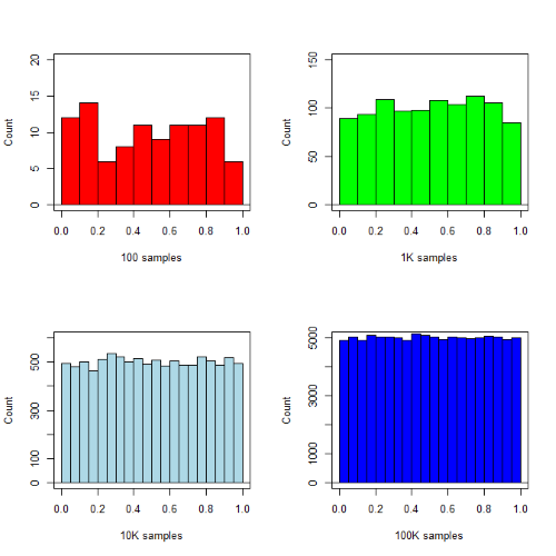
Figure 1. Histograms of runif results with 100, 1K, 10K, and 100K numbers of values to be generated
Looks pretty uniform. A property of random numbers is that history should not influence the future, i.e., no autocorrelation. We can check using the acf() function (Fig. 2).
par(mfrow = c(2, 2))
acf(myUniformH, main="100")
acf(myUniform1K, main="1K")
acf(myUniform10K, main="10K")
acf(myUniform100K, main="100K"
dev.off()
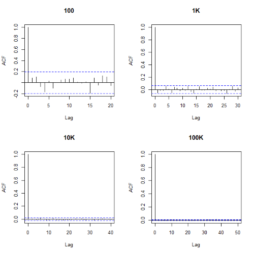
Figure 2. Autocorrelation plots of runif results with 100, 1K, 10K, and 100K numbers of values
Correlations among points are plotted versus lag, where lag refers to the number of points between adjacent points, e.g., lag = 10 reflects the correlation among points 1 and 11, 2 and 12, and so forth. The band defined by two parallel blue dashed lines
Questions
- Use
set.seed(123)and repeatrunif(10)twice. Confirm that the two sets are different (do not set seed) or the same whenset.seedis used. R hint: use functionidentical(x,y), where x and y are the two generated samples. This function tests whether the values and sequence of elements are the same between the two vectors.
Chapter 19 contents
- Introduction
- Jackknife sampling
- Bootstrap sampling
- Monte Carlo methods
- Ch19 References and suggested readings
List of R commands
List and links to R commands (followed with parentheses), R packages, and R Commander menu selections
Link to terms Index Mike’s Biostatistics Book
Click on name of command to take you to chapter and section where the command is presented. Note you may need to scroll down on the page to view the code and command.
R commands
.RProfile
aov()
ave()
c()
chisq.text()
data()
data.frame()
Dotplot()
dplyr()
epiR; Ch07.2
epi.conf()
exp()
geosd()
head()
help()
kruskal.test()
log()
mad()
mean()
median()
names()
pchisq()
plot()
pnorm()
pnormGC()
qchisq()
qt()
quantile()
range()
rank()
require()
RGUI menu: File → New script
round()
scan()
sd()
seq()
stack()
summary()
table()
t.test()
tapply()
with()
R Commander menu selections
Rcmdr: Distributions → Continuous distributions → Normal distribution → Normal quantiles…
Rcmdr: File → Exit
Rcmdr: Manage Mac OS X app nap for R.app…
/MD
20.13 – How to get the distances from a distance tree
Introduction
Extract the patristic distance, the sum of the branch lengths that link two nodes in a tree, for each pair of species.
This distance — see our Chapter 16.6 – Similarity and Distance— is the proportion (p) of amino acid (or nucleotide for DNA or RNA) sites at which the two sequences to be compared are different. It is obtained by dividing the number of amino acid differences by the total number of sites compared. It does not make any correction for multiple substitutions at the same site or differences in evolutionary rates among sites. On a gene tree (Fig. 1), distances are the lengths of the branches connecting the taxa. We want to know how different are two species for the given protein? That’s the distance between them in proportion of amino acid sites that are different by total number compared.
Example
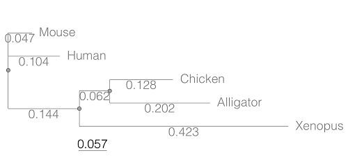
Figure 1. A gene tree of the product (protein HBA1) with five species.
Here’s the Newick format for the tree (HBA1.nwk)
(Mouse:0.0474516,Human:0.104063,((Chicken:0.127652,Alligator:0.202421):0.0616593,Xenopus:0.422801):0.143939);
R code to extract distances and output sorted, pairwise comparisons to a text file
library(ape)

# Create a function
getDis <- function(tree, tips) {
     myTree <- cophenetic(tree)
     myTree <- myTree[,tips]
     xy <- t(combn(colnames(myTree), 2))
     xy <- xy[order(xy[,1], xy[,2]),]
     myOut <- data.frame(xy, myTree[xy])
     colnames(myOut) <- c("Spp1", "Spp2", "Distance")
   return(myOut)
}

# Read a tree file, Newick format
tree5 <-read.tree(text="(Mouse:0.0474516,Human:0.104063,((Chicken:0.127652,Alligator:0.202421):0.0616593,Xenopus:0.422801):0.143939);")

# get taxa names from the tree file
all.tips <- tree5$tip.label; all.tips

# Run the function
myDis <- getDis(tree5, all.tips)

# Check the output
head(myDis)

# Create the results file
write.csv(myDis, file = "my_out.txt")
Example output from head(myDist)
       Spp1    Spp2  Distance
1 Alligator Xenopus 0.6868813
2 Chicken Alligator 0.3300730
3 Chicken   Xenopus 0.6121123
4 Human   Alligator 0.5120823
5 Human     Chicken 0.4373133
6 Human     Xenopus 0.6708030
The function sorts first by Spp1, then by Spp2.
Molecular clock plot
Collect divergence times from timetree.org
| Spp1 | Spp2 | Time (median MYA) |
| Alligator | Xenopus | 352 |
| Chicken | Alligator | 245 |
| Chicken | Xenopus | 352 |
| Human | Alligator | 319 |
| Human | Chicken | 319 |
| Human | Xenopus | 352 |
A scatterplot of distance HBA protein sequence by log10-transformed millions of years ago divergence time shown in Figure 2. Note, although tempting, calculating the slope from a linear regression to estimate the rate of evolution would not be appropriate without accounting for the lack of independence of the data (see Phylogenetically independent contrasts). Better methods exist, including calculating rate of change after fitting a model that assumes a strict clock vs relaxed clock.
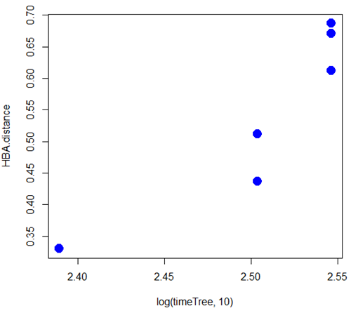
Figure 2. Scatterplot HBA distance by logMYA divergence time
Questions
[pending]
Suggested readings
Bevan, R. B., Lang, B. F., & Bryant, D. (2005). Calculating the evolutionary rates of different genes: a fast, accurate estimator with applications to maximum likelihood phylogenetic analysis. Systematic biology, 54(6), 900-915.
Chapter 20 contents
- Additional topics
- Area under the curve
- Peak detection
- Baseline correction
- Surveys
- Time series
- Dimensional analysis
- Estimating population size
- Diversity indexes
- Survival analysis
- Growth equations and dose response calculations
- Plot a Newick tree
- Phylogenetically independent contrasts
- How to get the distances from a distance tree
- Binary classification
- Meta-analysis
/MD
R packages
What’s on this page?
- How to add packages to base R installation.
- How to select a CRAN mirror site.
- Steps for package installation from selected CRAN mirror site.
- How to load and unload a package.
- How to update installed packages following an upgrade of R.
- List of R packages used in the Mike’s Biostatistics Book.
The instructions on this page chiefly apply to an installation of R on a local computer, Linux, macOS, or winPC. Running R in the cloud (eg, Google CoLab) also requires installing and loading packages, but many of the other instructions on this page do not apply. Look for the CoLab, skip this step: statement; instructions lacking this disclaimer should apply to CoLab. After a skip this step: statement, I’ll start the new section with Applies to all.
Add packages to base R installation
CoLab, skip this step: it is not necessary to set a mirror site for Google CoLab.
Installing R packages is straightforward, assuming the package is part of CRAN. Select a CRAN mirror site, eg, 0-Cloud, RStudio’s mirror site.
chooseCRANmirror()
To find out what CRAN mirror was set for the current session use
findCRANmirror()
A list of mirror sites is stored on your computer once R is installed, see CRAN_mirrors.csv in the doc folder, eg, ~/R-4.3.1/doc.
Applies to all. Once the CRAN mirror is selected, and assuming you have the name of the package, eg, package.name, then
install.packages("package.name")
will work.
Useful additional command options include
install.packages("package.name", dependencies=TRUE)
which will also download and install any additional packages required. And
install.packages("package.name", quiet=TRUE)
which cuts down on the amount of screen output during installation.
If you receive the warning message
Warning: package 'package.name' is not available (for R version 4.3.2)
While it is possible the package has not yet become available, first double-check for typos.
Another warning message may be that a binary version is available, but a more recent source version is available, prompted by the question,
Do you want to install from sources the package which needs compilation?
In most cases, no is the answer. R will install a previous binary version. In order to install from source, RTools must be installed.
Note 1: Do not install RTools if running R in the cloud (eg, Google CoLab). The R environment on CoLab is already set.
RTools contains software tools needed to build some R packages on WinPC.
Start, stop, or remove package
Applies to all. library("package name") is used to start a package. If a package is to be called in a function, then use require("package name"). If the called package is not installed, library() will exit with an error message whereas the function will continue to run if require() is used.
To unload a package without stopping current R session, try detach("package name") or unloadNamespace("package name"). The command remove.packages("package name") will uninstall a package from R.
Update R packages after installing new R version
CoLab, skip this step: After updating to new version of R you’ll need to download and update the user installed packages again. If you are running RStudio, see instructions here. For Win11 users you can download and run a package called installr, for macOS users download and install updateR, which will assist you to update R packages.
I prefer to run a script I modified from R-Bloggers.com. This script works on any operating system, but updates only CRAN packages (eg, not devtools github or Bioconductor packages). For github, try . dtupdate. For Bioconductor, see BiocManager::install() ).
Before installing the new version of base R, start up your current R installation and set your working directory, setwd(). Enter the following script to gather and save all installed R packages. Select CRAN mirror when prompted.
tmp <- installed.packages()
installedpkgs <- as.vector(tmp[is.na(tmp[,"Priority"]), 1])
save(installedpkgs, file="installed_old.rda")
Shutdown R, then install and start the new version of R (see Install R for help).
In the new version of R, set your working directory as above. Enter the following script
load(file="installed_old.rda")
tmp <- installed.packages()
installedpkgs.new <- as.vector(tmp[is.na(tmp[,"Priority"]), 1])
missing <- setdiff(installedpkgs, installedpkgs.new)
install.packages(missing)
update.packages(ask=FALSE)
Should be good to go. You can remove old R version installation.
Note 2: to check installed packages, just view the object installedpkgs created earlier.
R packages used in Mike’s Biostatistics Book
list updated 12 August 2024
| package | chapter |
|---|---|
| agRee | 16.5 – Instrument reliability and validity |
| ape | 20.11 - Plot a Newick tree |
| baseline | 20.3 - Baseline correction |
| BiocManager | 20.11 - Plot a Newick tree |
| Bioconductor | 20.11 - Plot a Newick tree |
| BiodiversityR | 5.6 - Sampling from Populations |
| boot | 19.2 - Bootstrap sampling |
| bootstrap | 19.1 - Jackknife sampling |
| BSDA | 11.4 - Two sample effect size |
| cairoDevice | 13.3 – Test assumption of normality |
| car | 4.3 - Box plot |
| carData | 4.1 - Bar (column) charts |
| cholera | 2.3 - A brief history of (bio)statistics |
| clipr | 4 – How to report statistics |
| combinat | 6.3 - Combinations and permutations |
| confintr | 19.2 - Bootstrap sampling |
| contingencytables | 9.6 – McNemar’s test |
| correlation | 16.6 - Similarity and Distance |
| cranlogs | 2.2 – Why do we use R Software? |
| datasets | 4.5 - Scatter plots |
| digitize | 12.3 - Fixed effects, random effects, and ICC |
| drc | 20.10 - Growth equations and dose response calculations |
| effectsize | 12.5 – Effect size for ANOVA |
| effsize | 11.4 - Two sample effect size |
| epiR | 5.4 - Clinical trials |
| epitools | 7.4 – Epidemiology: Relative risk and absolute risk, explained |
| exact2x2 | 9.6 – McNemar’s test |
| factoextra | 20.6 – Dimensional analysis |
| findpeaks | 20.2 - Peak detection |
| forecast | 20.5 - Time series |
| geepack | 20.1 - Area under the curve |
| geeM | 20.1 - Area under the curve |
| geodist | 16.6 - Similarity and Distance |
| ggplot2 | 4.1 - Bar (column) charts |
| ggtree | 20.11 - Plot a Newick tree |
| gplots | 4.1 - Bar (column) charts |
| gtools | 6.3 - Combinations and permutations |
| GrapheR | 4.10 - Graph software |
| HH | 12.4 - ANOVA from "sufficient statistics" |
| HistData | 3.2 - Measures of Central Tendency |
| lattice | 4.10 - Graph software |
| lmboot | 19.1 - Jackknife sampling |
| irr | 12.3 - Fixed effects, random effects, and ICC |
| MASS | 12.4 - ANOVA from "sufficient statistics" |
| Matrix | 20.1 - Area under the curve |
| mcp | 12.6 - ANOVA posthoc tests |
| MESS | 20.1 - Area under the curve |
| mlr3misc | 8.2 – The controversy over proper hypothesis testing |
| modeest | 3.2 - Measures of Central Tendency |
| multcomp | 12.6 - ANOVA posthoc tests |
| NCStats | 3.3 - Measures of dispersion |
| nlopt | 20.10 - Growth equations and dose response calculations |
| nortest | 13.3 – Test assumption of normality |
| PairedData | 10.3 – Paired t-test |
| peakDetection | 20.2 - Peak detection |
| Phylotools | 20.11 - Plot a Newick tree |
| Phytools | 20.11 - Plot a Newick tree |
| plotly | 4.10 - Graph software |
| plyr | 4.1 - Bar (column) charts |
| polychor | 16.4 – Spearman and other correlations |
| propCIs | 7.6 - Confidence intervals |
| psa | 20.6 – Dimensional analysis |
| psy | 12.3 - Fixed effects, random effects, and ICC |
| psych | 3.2 - Measures of Central Tendency |
| pwr | 11.5 - Power analysis in R |
| random | 6.6 - Continuous distributions |
| rattle | 13.3 – Test assumption of normality |
| Rcmdr | 1.1 – A quick look at R and R Commander |
| RcmdrMisc | 1.1 – A quick look at R and R Commander |
| RcmdrPlugin.EBM | 4.4 - Mosaic plots |
| RcmdrPlugin.EZR | 11.5 - Power analysis in R |
| RcmdrPlugin.HH | 12.4 - ANOVA from "sufficient statistics">/a> |
| RcmdrPlugin.KMggplot2 | 4.1 - Bar (column) charts |
| RcmdrPlugin.mosaic | 4.4 - Mosaic plots |
| RcmdrPlugin.survival | 20.9 - Survival analysis |
| Rcolorbrewer | 4.4 - Mosaic plots |
| reshape2 | 4.6 - Adding a second Y axis |
| rgl | 18.1 - Multiple Linear Regression |
| Rmisc | 3.5 - Statistics of error |
| ROCR | 20.1 - Area under the curve |
| rptR | 12.3 - Fixed effects, random effects, and ICC |
| RGtk2 | 13.3 – Test assumption of normality |
| season | 20.5 – Time series |
| shotGroups | 3.5 - Statistics of error |
| stats | 4 – How to report statistics |
| survival | 3.1 - Data types |
| tanggle | 20.11 - Plot a Newick tree |
| Ternary | 4.8 - Ternary plots |
| testequavar | 13.4 – Tests for Equal Variances |
| tidyverse | 4.3 - Box plot |
| tigerstats | 8.4 – Tails of a test |
| timeseries | 20.5 – Time series |
| TOSTER | 16.1 – Product moment correlation |
| vegan | 20.8 - Diversity indexes |
| WRS2 | 3.3 – Measures of dispersion |
6.8 – Moments
Introduction
We care about the shape of data distribution because it can impact statistical inference. If the shape of the observed distribution differs from the standard, eg, normal, then one option is to transform the data (see Chapter 13 – Assumptions of parametric tests).
Moments are used to describe the shape of a distribution. For those of you who remember your calculus, moments were discussed as a method to find the center of mass, or balancing point (Herman and Strang 2018). For distributions, the center and shape moments follow from the expected value of the probability function.
Note 1: Expected value of a statistic is calculated by multiplying the likelihood of each possible outcome in a sample space, then adding up all of those values. From probability theory it is the weighted average of the outcomes of a random variable. A simpler way to think of the expected value is that if one were to guess the height of a person, the expected value is the average height of the population from which the person would be selected.
Four moments apply for describing the shape of a distribution. The 1st moment describes the middle, the 2nd describes the spread from the middle, the 3rd describes symmetry about the middle, and the 4th describes the shape, whether peaked and sharp (leptokurtic), or broad and flattened (platykurtic).
Equations for the moments
Over the years, several equations have been proposed to estimate skewness and kurtosis. The above formulas are just one example from the list (Joanes and Gill 1998).
Pearson’s standardized moments:
![\begin{align*} \frac{\mu_{n}}{\sigma ^{n}}\equiv \frac{E\left [ X-\mu \right ]^{n}}{\sigma ^{n}} \end{align*}](https://biostatistics.letgen.org/wp-content/ql-cache/quicklatex.com-9b3275c780ca09d2cddbb8a57f099063_l3.png "Rendered by QuickLaTeX.com")
where E is expected value of random variable. The expected value concept follows from rules of probability — basically, the average of large number, n, of X.
Four moments can be used to describe the shape of a distribution.
1st moment, μ (mean): population mean, 3.1 – Measures of Central Tendency
2nd moment, σ2 (variance): population variance, 3.2 – Measures of dispersion
3rd moment, ![]() (skew):
(skew):
![\begin{align*} \frac{\mu_{3}}{\sigma ^{3}}=\frac{\sqrt{n\left ( n-1 \right )}}{n-2}\left [ \frac{\frac{1}{n}\sum \left ( X-\mu \right )^3}{\left ( \frac{1}{n}\sum \left ( X-\mu \right )^2 \right )^3} \right ] \end{align*}](https://biostatistics.letgen.org/wp-content/ql-cache/quicklatex.com-a2b47ea0fc3a005dc31f6edfb318f001_l3.png "Rendered by QuickLaTeX.com")
4th moment, ![]() (kurtosis):
(kurtosis):

Estimating moments in R and R Commander
Consider results for more than a thousand runners who completed a 5K timed run (Fig 1).
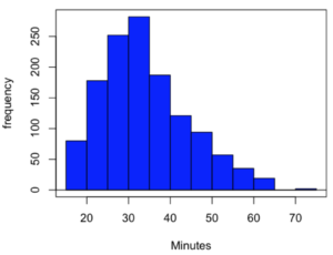
Figure 1. Histogram finishing times in minutes for 1307 runners at 2016 Banana 5K.
The task is to describe the moments for the 5K data set.
Recall: The first moment is the mean. The second moment is the variance. The third moment is skewness. And the fourth moment is kurtosis.
In R Commander, we select Statistics → Summaries → Numerical summaries…, which brings up a popup menu. First, select the variable, in this case Minutes, from the Data tab (not shown). Next, click on Statistics tab to choose options (Fig 2).
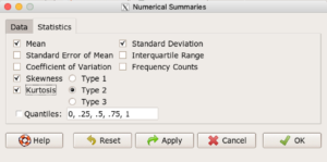
Figure 2. Rcmdr Numerical summaries Statistics tab.
For estimates of the moments, check Mean, Standard Deviation, Skewness, and Kurtosis.
Note 2: R Commander gives you the choice among three different Types of skewness and kurtosis. The default is type 2 and that’s the one you should go with. Type 1, the classical method which include the equations provided on this page, corresponding to definitions dating back to the 1940s. Type 2 is the default in R and corresponds to equations used by other professional statistics package (SAS, SPSS). Type 3 is used by other statistical packages (eg, Minitab). For large sample size, the different types will tend to agree. Caution applies to smaller data sets — the different types may disagree (Joanes and Gill 1998), although only for the third and fourth moments.
Large sample size, n = 1307
Type 1
    mean       sd  skewness    kurtosis    n
34.42999 10.31437 0.6159258 -0.01593882 1307
Type 2
    mean       sd  skewness    kurtosis    n
34.42999 10.31437 0.6166337 -0.01139521 1307
Type 3
    mean       sd skewness    kurtosis    n
34.42999 10.31437 0.615219 -0.02050335 1307
Small sample size
To test the claim about sample size and the moment statistics, draw a random sample of 30 from the larger data set. Sample without replacement
sample.banana <- data.frame(sample(banana5K$Minutes, 30, replace = FALSE))
I forgot to specify a new variable name, so R used the whole command as the variable name. I could go back and fix my function call, or simply rename the variable as follows
names(sample.banana)[c(1)] <- c("Minutes")
The random sample yielded a distribution (Fig 3).
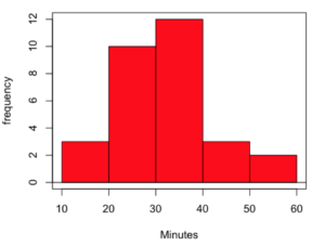
Figure 3. Histogram finishing times in minutes for random sample of 30 drawn from 1307 runners at 2016 Banana 5K.
Repeat Numerical summaries on small data set, n = 30
Type 1
    mean       sd  skewness  kurtosis  n
33.16667 10.00373 0.5538637 0.5024438 30
Type 2
    mean       sd  skewness  kurtosis  n
33.16667 10.00373 0.5834511 0.8276415 30
Type 3
    mean       sd  skewness  kurtosis  n
33.16667 10.00373 0.5264025 0.2728392 30
Conclusion: We can compare consistency of the estimators by calculating coefficient of variation. The three types of skewness estimators differed by only 1% and 5% for large and small sample size, respectively. In contrast, the three types of kurtosis estimators differed by 29% and 52% for large and small sample size, respectively.
Questions
- Explore the consistency of skewness and kurtosis estimates by calculating and comparing coefficient of variation estimates. R Commander provide a nice way to draw randomly from various defined distributions. Draw two data sets of 15 (small) and 1000 (large), from the chi-square distribution (1 degree of freedom) and a minimum of one other continuous distribution.
Example, draw random sample of 1000 from chi-square distribution. Rcmdr: Distributions → Continuous distributions → Chi-squared distribution → Sample from chi-squared distribution... (Fig 4).
Enter name for the variable, enter degrees of freedom (e.g., 1), number of samples (e.g., 1000), and number of observations (variables, columns). Leave Sample means checked under data sets.
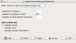
Figure 4. Screenshot Rcmdr menu: Sample from Chisquare distribution.
This results in a new data set. Get “moments” from Numerical summaries and calculate coefficient of variations. Which moments have the most consistency regardless of the kind of distribution.
- Make histograms for each of your created data sets. Describe what you see about the shape of the plotted distributions.
Quiz Chapter 6.8
Moments
Chapter 6 contents
- Introduction
- Some preliminaries
- Ratios and proportions
- Combinations and permutations
- Types of probability
- Discrete probability distributions
- Continuous distributions
- Normal distribution and the normal deviate (Z)
- Moments
- Chi-square (Χ2) distribution
- t distribution
- F distribution
- References and suggested readings
Install R
This page has 30 images
Introduction
The first time installing R can seem intimidating. To start, be clear about the overall goal of the procedure: providing the student with an accessible environment for solving statistics problems.
In brief, this page explains how to get R set up on your computer. First, you need to download the R installer from the official CRAN website. When you run the installer,in general, accept the default choices. However, for Windows users, it’s important to right-click the file and choose “Run as administrator.” This step ensures that R has the proper permissions to install correctly and avoids problems with user access later on. Once installed, you can open R and test it by typing a simple command like `2 + 2` in the console to confirm everything is working.
The flow chart presented in Fig 1 suggests a way to orient the student to solving the task. First, understand which type of computing environment you have available. Second, if a macOS, then additional software (XQuartz) is required to provide full function to the R software. Third, download and install the base R software appropriate for the computer system.
Figure 1 suggests an R installation flow chart.
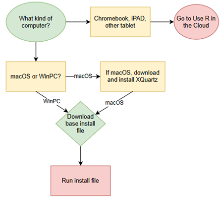
Figure 1. Suggested flow chart for R installation.
Note 1: I skipped Linux in the flow chart — I’m working on the assumption that Linux users are more comfortable installing 3rd party software. However, some notes on R installs on Linux distros are included on this page.
It’s possible to follow the steps in Figure 1, accepting all default options presented along the way, to end up with a working R environment. As with many software processes, there are choices beyond defaults that can be made to improve the software use.
This page presents a detailed guide about how to install R onto your computer — this is referred to as building a local development environment or LDE. Additional install R help was provided in Chapter 1.1 – A quick look at R and R Commander.
Instructions for RStudio are also provided (optional for BI311 students). A guide to install R Commander is provided in Install R Commander.
Instructions for how to run R via a “cloud computing” (serverless) option — a remote development environment — are also provided, Use R in the Cloud.
For help upgrading installed packages after upgrading new R version, see R packages.
Note 2: Installation guides quickly become outdated. This page was created first in September 2019 and last updated August 2025 and describes working installation protocols at that time. As of August 2025, R -4.5.1 was current version. Instructions for Win10 and Win11 are the same. Instructions for Intel-based macOS are the same; with Apple’s switch to ARM64 (M1, M2, M3, M4), changes have been made. Going forward, the instructions on this page, but not my videos — version numbers need to be updated in the videos, are likely to be the same for new R versions. And wow! Search Google or Bing for “how to install R,” options in the millions. Ultimately the best source is in the R installation and administration manual.
Per usual caveat about this page of instructions: my advice is offered for instructional purposes and in no way implies warranty against damage or guarantee of success.
Run R on your computer (LDE install)
CoLab, skip this step: Instead, go to Use R in the cloud.
So why in this day in age should you install and build R on your own computer? The remote options to run R in the cloud are a wonderful option, convenient: you can access anywhere you have internet, from any device that connects to the internet. It’s easy to share and work together on projects, particularly those based on Jupyter Notebooks.
I think the main benefits to a local installation is it’s a more efficient environment to work in — you have control of everything and, provided your PC has power, a working R install on your computer will always be available to you. Since you can control the update cycle for your computer, you won’t run into times you cannot access the remote server to work on your project. Testing code is faster on a local install, feedback — think error messages — apply to your installed version. And, while remote R servers may come with low initial costs to students, any significant use will quickly require paid accounts. As a reminder, the good folks at the R-project continue to offer R as free software. All you need to do is work through the install process.
Start at the R-project homepage, r-project.org. To download software, first click on CRAN link, located on left hand side of the screen (here, highlighted by green arrow, Fig 2).
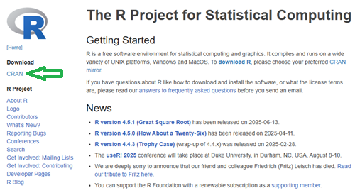
Figure 2. Screenshot homepage for R-project.org.
Figure 3 shows a screenshot of the CRAN mirror page. The idea is to select the mirror site closest to your location. In Hawaiʻi, that’s likely to be any of the sites in California. However, I recommend selecting the first in the list, 0-cloud, at cloud.r-project.org (highlighted by green arrow, Fig 3).

Figure 3. Screenshot of portion of R-Project CRAN mirror page.
Note 3: After installing R, see this page to learn how to set the CRAN mirror.
After selecting the mirror site, the download page is presented (Fig 4). Click on the link that corresponds to your computer system (Linux, macOS, or Windows).
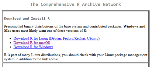
Figure 4. Screenshot of portion of base R download page.
Once the installation file is located onto your computer, proceed to install base R.
Detailed instructions
For screenshots of installation steps on WinPC, see Win10/11 setup, screenshots
- Windows PCs, download the base application from selected CRAN Mirror site, select Download R for Windows, and install the R software as you would any other software. All of you are likely to have the 64-bit version of Windows 11, so install the 64-bit version of R. Follow the instructions as they are presented. Screenshots of the install process are available at the end of this page (click here or scroll down to Win11 setup, Screenshots).
- Current versions of Microsoft Windows come in several flavors, the simplest distinction is between home and pro. R runs perfectly well on both.
- Windows 10 is reaching end of life cycle.
- Some inexpensive Microsoft Windows PCs are built on ARM64, not Intel or AMD64 CPU. Thus, installing R and or RStudio may prove problematic.
- Also note: Windows in S mode only run applications from the Microsoft store. To install R, you first may need to switch out of S mode (see Microsoft FAQ about S mode).
- You should install R with Administrator privileges. Highlight the install file, right-click the file, and select “Run as administrator” from the popup menu.
- When you first try to run R you may get a popup screen “Windows protected your PC,” locate and click on the “More info” link and select “Run anyway.”
- This in no way will harm your computer — provided you have downloaded from official sites. R is a verified program. Microsoft has taken an aggressive line on developers and favors apps that are part of their app store.
- It is advisable to confirm for yourself: check the md5sum against the fingerprint on the CRAN server
- When prompted, I recommend that you change the install directory to root folder, e.g.,
C:\R\R-4.5.1. This will allow for installation of packages to the common library as opposed to a personal library.- I recommend this change because of how Windows assigns home folders. During initial setup Windows 10 prompted you to choose a username and whether you wanted your work stored locally or in your OneDrive folder. A worse case scenario? You select a username with spaces, e.g.,”Mike Dohm,” and you selected OneDrive. Both will cause challenges later for running and or installing packages for R.
- If you install R anywhere but the default Program files folder on your Win10/11 PC, chances are you will need to add the folder containing the executable, r.exe, to you path.
- Search: “env”
- Open “Edit the system environment variables” in the Control Panel
- Click Advanced tab, then click on Environment Variables… button (lower right of panel)
- Under System variables, scroll to and select Path.
- Click Edit… button, then click New button.
- Type in the path to the folder containing R.exe. That’s likely to be C:\R\R-4.5.1, assuming R-4.5.1 is the latest version of R installed on your computer.
- If you install R anywhere but the default Program files folder on your Win10/11 PC, chances are you will need to add the folder containing the executable, r.exe, to you path.
- I made a video for you. Video is about 26 minutes long; at 22 minute mark, video includes how to install R Commander (instructions provided Install R Commander).
- Apologies for the production quality — videos are not my thing.
- I recommend this change because of how Windows assigns home folders. During initial setup Windows 10 prompted you to choose a username and whether you wanted your work stored locally or in your OneDrive folder. A worse case scenario? You select a username with spaces, e.g.,”Mike Dohm,” and you selected OneDrive. Both will cause challenges later for running and or installing packages for R.
- Current versions of Microsoft Windows come in several flavors, the simplest distinction is between home and pro. R runs perfectly well on both.
For screenshots of installation steps on WinPC, see MacOS setup, screenshots
- macOS PCs, first you must download and install XQuartz from https://www.xquartz.org. Best to restart your mac after installing XQuartz then proceed to install R.
After installing XQuartz, then return to https://cran.r-project.org, select Download for Mac(OS) X, and run the installer. Screenshots of the install process are available at the end of this page (click here or scroll down to Macos setup, Screenshots).- As of August 2025, be advised that there are two distinct R versions for your MacBook or iMac.
- For MacBook or iMac with Apple’s M1 or M2 ARM chip sets, download and install
R-4.5.1-arm64.pkg.- If you recently purchased a new MacBook or iMac (2020 to present), then you probably have the M2 or M3 chipset (check by clicking the Apple icon, then selecting About this Mac or System Information (
/Applications/Utilities/System Information.app)). - XQuartz version 2.8.5 works on macs with either the M1 or Intel chipsets.
- If you recently purchased a new MacBook or iMac (2020 to present), then you probably have the M2 or M3 chipset (check by clicking the Apple icon, then selecting About this Mac or System Information (
- For older MacBook or iMacs with Intel processors, download
R-4.5.1-x86_64.pkg. Depreciated 8/4/2021: Be advised that these instructions are for Intel-based macs. At the time of writing these instructions (April 2021), the installation of XQuartz and R should work on new M1-based macs. At the time of this writing (April 2021), however, R will not run natively on your M1 mac. It will run using Rosetta 2, an emulator that is included with your M1 mac. The R folks are busy working on a version that will run natively, which may be ready within a few months.
- For MacBook or iMac with Apple’s M1 or M2 ARM chip sets, download and install
- At the completion of the install process, don’t forget to drag the R app to your Applications folder.
- When you first try to run R, you may get a popup screen which provides no option to start the app, and perhaps even a rather ominous option to move the app to Trash. Just close the warning message and right-click on the R app. A new screen pops up, which looks very much like the previous warning, but now you will see and option to open the app. Click on open to start R.
- Like the message to Windows PC users, bypassing Apple’s Gatekeeper to run R in no way will harm your computer — provided you have downloaded from official sites — R is a verified program. Apple has taken an aggressive line on developers and favors apps that are part of their app store.
- As of August 2025, be advised that there are two distinct R versions for your MacBook or iMac.
- LINUX distros. If your PC platform is Linux, then you should be comfortable with installation and updating of software. R base is already included in Debian distributions (e.g., Mint, Ubuntu). See https://cloud.r-project.org/ for additional instructions.
- For Chromebook users, if you can install a Linux subsystem, then you can also install and run R. For instructions to install R see Levi’s excellent writeup at levente.littvay.hu/chromebook/.
Note 4: To install up-to-date R and RStudio, your Chromebook needs to have Intel or AMD CPU; my ASUS Chromebook has an ARM64 processor (MediaTek mt8183), and Levi’s instructions don’t apply. As of January 2024 I am pushing the installation process a bit on my little Chromebook and have successfully created the Linux container (Debian 11, Bullseye) and installed base (and development) R version (4.0.4) included with the Linux distribution. Stay tuned — I’ll update progress with installing an R environment on ARM64-based Chromebook.
Update August 2025 — no change, very challenging to get R environment running and updated on ARM64 Chromebook. RStudio not possible.
Test R
For both macOS and Windows PCs, successful installation of R on your computer installs base R programming language and a simple graphical user interface. Test your install by running code in the terminal (one line at a time) or via script:
- Rgui.exe (Windows PC)
- File → New script
Enter code in script editor, e.g.,
myX <- c(1,2,3,4)
myY <- c(5,10,15,20)
plot(myY,myX)
- Run code: Ctrl+R
Figure 5 shows screenshot of R running on WinPC. RGui.exe (1), script editor (2), and results of plot() (3) on WinPC.
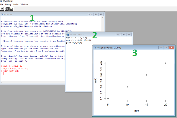
Figure 5. Screenshot of RGui.exe (1), script editor (2), and results of plot() (3) on WinPC.
- R.app (macOS): run code in the terminal or via script
- File → New Document
Enter code in script editor, e.g.,
myX <- c(1,2,3,4)
myY <- c(5,10,15,20)
plot(myY,myX)
- Run code: Cmd+Enter
Figure 6 shows screenshot of R running on macOS. R.app (1), script editor (2), and results of plot() (3).
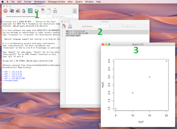
Figure 6. Screenshot of R.app (1), script editor (2), and results of plot() (3) on macOS.
Many of you would like a video. Do a little search and you’ll find plenty, although most are also showing how to install RStudio in addition to base R.
Note 5: For my Biostatistics class, BI311, we typically will run R and use R Commander for scripting, without RStudio.
For BI311, we also use R Commander package
R Commander is a package that adds function to R; it provides a familiar point-and-click interface to R, which allows the user to access functions via a drop-down menu system (Fox 2017).
Go to Install R Commander guide.
Personalize R startup
To add function to R, you’ll download many R packages. These, too, are stored at the mirror sites. Each time you run install.packages(), R will ask for the mirror site. The R app on Windows pops up a long selection box; macOS R.app is a bit more friendly, but regardless, it’s best to choose a mirror site at the beginning of a session. At the R prompt, type and submit the command
options(repos = c(CRAN = "https://cloud.r-project.org"))
this will remain in effect for the current R session.
To make the change permanent, add to .Rprofile — a hidden file — in your personal home directory
local({
r <- getOption("repos")
r["CRAN"] <- "https://cloud.r-project.org"
options(repos = r)
})
If you use textedit or notepad, make sure to return after the }); the file requires an empty new line to run.
Restart R, then enter at the prompt
file.exists("~/.Rprofile")
If you’ve created the Rprofile file correctly, R should repeat.
Run R from the terminal
Whether yours is a mac or win11 pc, you have a powerful computing environment lurking beneath the glossy graphic user interface. It’s called the terminal. The terminal is a place where text-based instructions may be written and submitted to command your computer to do something.
On win11 pc, the modern terminal is the Power Shell. Search “PowerShell,” then open Windows PowerShell. Alternatively, shortcut + X, then I key. This opens terminal in your home folder.
- You’ll want to navigate to your working folder, e.g., BI311 on the Desktop. Setting your working folder can be done in R of course, but at the terminal type the command “
cd \users\default\desktop\bi311“.
On macOS, Spotlight (search) “Terminal.app“. Alternatively, right-click on your working folder icon and select New terminal at Folder from the popup menu.
On Ubuntu Linux, shortcut keys + alt, then t key.
Open the included script editor
Use RStudio
Rstudio is a very popular data science IDE, specifically written for R programming. Therefore, if your goal is to become adept at R programming, go with RStudio. Like R Commander, Rstudio provides an environment to write an manage code, generate markdown reports, and importantly, manage files in R projects. Figure 7 shows a screenshot of RStudio: Clockwise, four panes: Source, Environment, Output, Console on WinPC. BI311 students, please note that I recommend use of R Commander and Google CoLab.
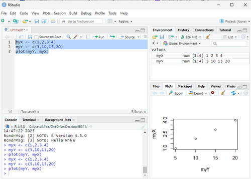
Figure 7. Screenshot of RStudio IDE.
Installation of RStudio desktop is straightforward.
Go to https://posit.co/download/rstudio-desktop/
Install R first. Since at this point you’ve likely already installed R, go directly to 2 (green box, Fig 8).
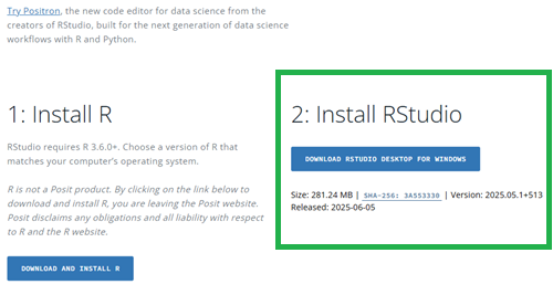
Figure 8. Screenshot RStudio desktop download page, current as of September 2025.
After downloading the installation software, double click the file to begin. Follow on screen instructions for your computer system.
Run R in the “Cloud”
If you do not wish to install R, or, if you have a Chromebook and, therefore cannot gracefully install R, then there are alternatives; Run R in the Cloud. I’ll list three ways to run R in the cloud for free. Go to Use R in the Cloud guide.
MacOS setup, Screenshots
Download R install package from R-project.org, then select the R install package from your Download folder (Fig 9).
Note 6: The following screenshots were for previous R version 4.1.1. As of Fall 2025, current R version is 4.5.1. The screenshots are consistent between the current and older versions of R on macOS.
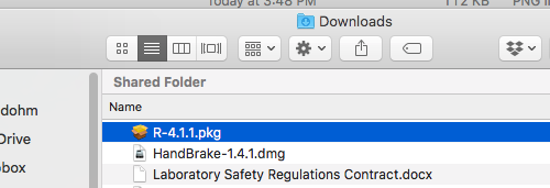
Figure 9. Screenshot — Find the R install file in your download folder.
First screen, R install for macOS (Fig 10). Select continue.
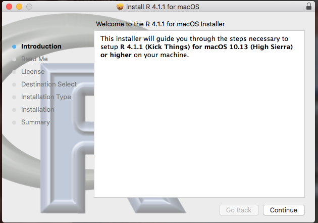
Figure 10. Screenshot: first instructions pop-up window.
Second screen, R install on macOS (Fig 11). Select continue.
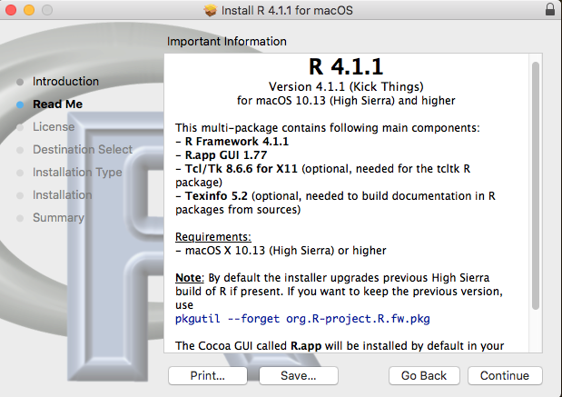
Figure 11. Screenshot: second instructions pop-up window.
Third screen, R install on macOS (Fig 12). Select continue.
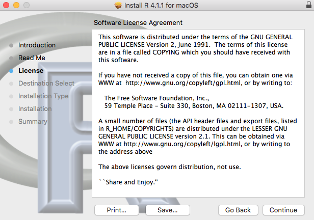
Figure 12. Screenshot: third instructions pop-up window.
Fourth screen, R install on macOS (Fig 13). Agree to continue.

Figure 13. Screenshot: fourth instructions pop-up window.
Fifth screen, R install on macOS (Fig 14). Select Install.
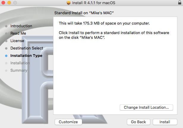
Figure 14. Screenshot: fifth instructions pop-up window.
Sixth screen, R install on macOS (Fig 15). Enter your username and password for your computer, then select Install Software.
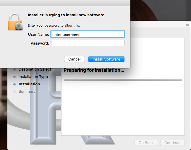
Figure 15. Screenshot: sixth instructions pop-up window.
Seventh screen, R install on macOS (Fig 16). Several screens will popup, reporting progress. Be patient!
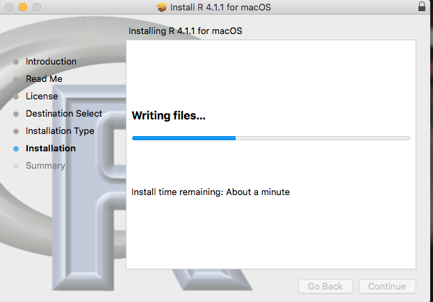
Figure 16. Screenshot: seventh instructions pop-up window.
Eighth and final screen, R install on macOS (Fig 17). Select close.
Figure 17. Screenshot: eighth and final instructions pop-up window.
Optional — Keep or discard the install file (Fig 18). I keep and then do manual delete after I’ve confirmed the installation.
Figure 18. Screenshot: MacOS will prompt with option to delete the installation file. This has no effect on the installation of R.
From Applications folder, start R.app. You should see the R Console (Fig 19).
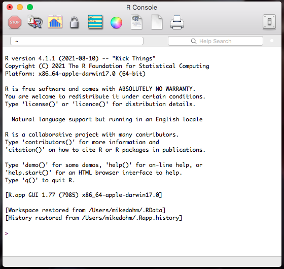
Figure 19. Screenshot: R Console in the R.app on macOS.
Wind10/11 setup, screenshots
Download from R-project.org, then right-click the R install package from your Download folder. Run as administrator (Fig 20).
Note 7: The following screenshots were for previous versions of R, 3.6.1 and 4.0.5. As of Fall 2025, current R version is 4.5.1. The screenshots are consistent between the current and older versions of R on Windows 10/11.
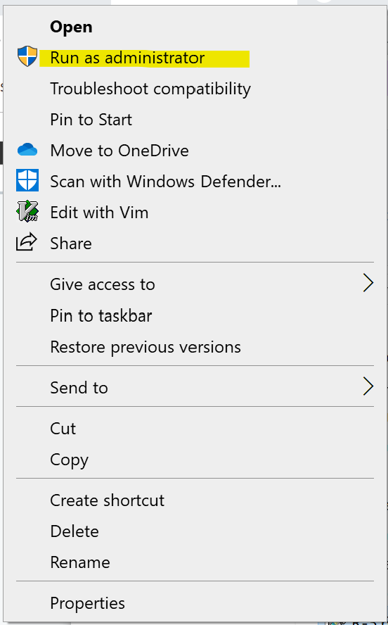
Figure 20. WinPC screenshot: Pop-up menu after right-click on the R installation file in windows Explorer.
First screen, select language (Fig 21). Select OK to continue
Figure 21. WinPC screenshot: first instructions pop-up window.
Second screen (Fig 22), click Next to continue
Figure 22. WinPC screenshot: second instructions pop-up window.
Third screen (Fig 23). Change the default location (show in the screenshot) to root folder, e.g., C:\R\R-4.5.1 (current version as of August 2025).
Figure 23. WinPC screenshot: third instructions pop-up window. Note — R-4.5.1 (current version as of August 2025).
Fourth screen (Fig 24). Change startup options. Select Yes (customized startup) to continue.
Figure 24. WinPC screenshot: fourth instructions pop-up window.
Fifth screen (Fig 25), select SDI — single document interface — not the default MDI — multiple document interface, then Next to continue.
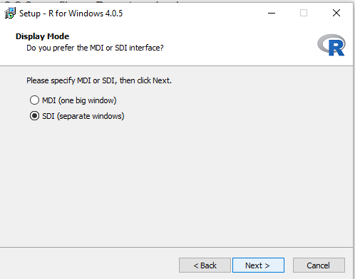
Figure 25. WinPC screenshot: fifth instructions pop-up window. Recommend setting to SDI.
Sixth screen (Fig 26), select HTML help, then Next to continue.
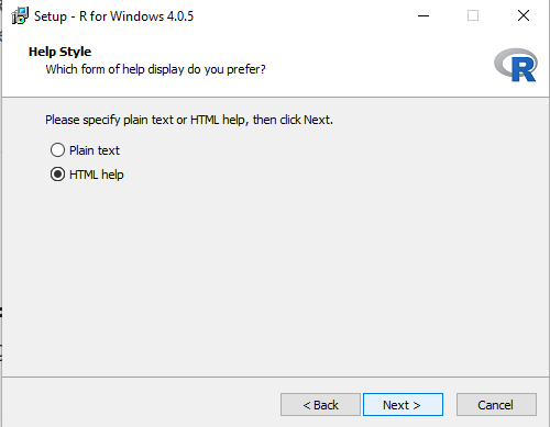
Figure 26. WinPC screenshot: sixth instructions pop-up window.
Seventh screen (Fig 27), leave start menu folder as is (R), then Next to continue.
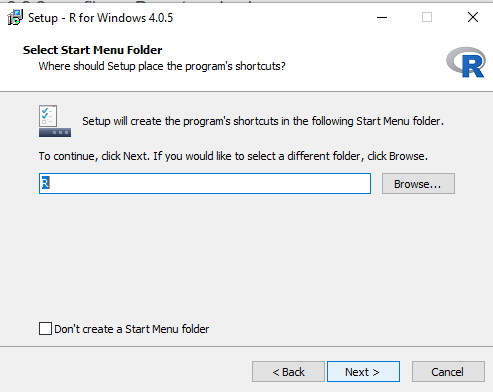
Figure 27. WinPC screenshot: seventh instructions pop-up window.
Eighth screen (Fig 28), check all boxes, then Next to continue.
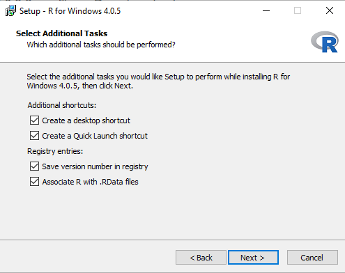
Figure 28. WinPC screenshot: eighth instructions pop-up window.
Ninth screen (Fig 29), a series of status updates during the installation.
Figure 29. WinPC screenshot: ninth instructions pop-up window.
Final screen (Fig 30), successful install.
Figure 30. WinPC screenshot: final instructions pop-up window — successful installation.
/MD
18.3 – Logistic regression
Introduction
We briefly introduced logistic regression in the previous chapter on nonlinear regression. We expand our discussion of logistic regression here.
Logistic regression is a statistical method for modeling the dependence of a categorical (binomial) outcome variable on one or more categorical and continuous predictor variables (Bewick et al 2005).
The logistic function may be used to transform a sigmoidal curve to a more or less straight line while also changing the range of the data from binary (0 to 1) to infinity (-∞,+∞). For event with probability of occurring p, the logistic function is written as
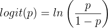
where ln refers to the natural logarithm.
This is an odds ratio. It represents the effect of the predictor variable on the chance that the event will occur.
The logistic regression model then very much resembles the same general linear models we have seen before.
![]()
In R and Rcmdr we use the glm() function to model the logistic function. Logistic regression is used to model a binary outcome variable. What is a binary outcome variable? It is categorical! Examples include: Living or Dead; Diabetes Yes or No; Coronary artery disease Yes or No. Male or Female. One of the categories could be scored 0, the other scored 1. For example, living might be 0 and dead might be scored as 1. (By the way, for a binomial variable, the mean for the variable is simply the number of experimental units with “1” divided by the total sample size.)
With the addition of a binary response variable, we are now really close to the Generalized Linear Model. Now we can handle statistical models in which our predictor variables are either categorical or ratio scale. All of the rules of crossed, balanced, nested, blocked designs still apply because our model is still of a linear form.
We write our generalized linear model

just to distinguish it from a general linear model with the ratio-scale Y as the response variable.
Think of the logistic regression as modeling a threshold of change between the 0 and the 1 value. In another way, think of all of the processes in nature in which there is a slow increase, followed by a rapid increase once a transition point is met, only to see the rate of change slow down again. Growth is like that (see Chapter 20.10 for related growth and related models). We start small, stay relatively small until birth, then as we reach our early teen years, a rapid change in growth (height, weight) is typically seed (well, not in my case … at least for the height). The curve I described is a logistic one (other models exist too). Where the linear regression function was used to minimize the squared residuals as the definition of the best fitting line, now we use the logistic as one possible way to describe or best fit this type of a curved relationship between an outcome and one or more predictor variables. We then set out to describe a model which captures when an event is unlikely to occur (the probability of dying is close to zero) AND to also describe when the event is highly likely to occur (the probability is close to one).
A simple way to view this is to think of time being the predictor (X) variable and risk of dying. If we’re talking about the lifetime of a mouse (lifespan typically about 18-36 months), then the risk of dying at one months is very low, and remains low through adulthood until the mouse begins the aging process. Here’s what the plot might look like, with the probability of dying at age X on the Y axis (probability = 0 to 1) (Fig 1).
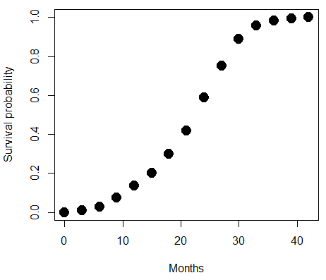
Figure 1. Lifespan of 1881 mice from 31 inbred strains (Data from Yuan et al [2012] available at https://phenome.jax.org/projects/Yuan2).
Note 1: I labeled Y axis labeled “Survival Probability”; “Inverse Survival Probability” would be more accurate.
We ask — of all the possible models we could draw — which model best fits the data? The curve fitting process is called the logistic regression. The sample data set is listed at end of this page (scroll down of click here). Create data.frame called yuan.
With some minor, but important differences, running the logistic regression is the same as what you have been doing so far for ANOVA and for linear regression. In Rcmdr, access the logistic regression function by calling the Generalized Linear Model (Fig 2).
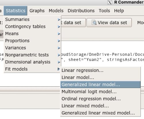
Figure 2. Access Generalized Linear Model via R Commander
R results
GLM.1 <- glm(cumFreq ~ Months, family=gaussian(identity), data=yuan)

> summary(GLM.1)

Call:
glm(formula = cumFreq ~ Months, family = gaussian(identity),
data = yuan)

Deviance Residuals:
     Min       1Q   Median      3Q     Max
-0.11070 -0.07799 -0.01728 0.06982 0.13345

Coefficients:
             Estimate Std. Error t value Pr(>|t|)
(Intercept) -0.132709   0.045757   -2.90 0.0124 *
Months       0.029605   0.001854   15.97 6.37e-10 ***
---
Signif. codes: 0 '***' 0.001 '**' 0.01 '*' 0.05 '.' 0.1 ' ' 1

(Dispersion parameter for gaussian family taken to be 0.008663679)

Null deviance: 2.32129 on 14 degrees of freedom
Residual deviance: 0.11263 on 13 degrees of freedom
AIC: -24.808

Number of Fisher Scoring iterations: 2
Rcmdr: Statistics → Fit models → Generalized linear model.
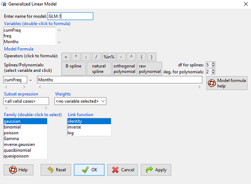
Figure 3. Screenshot Rcmdr GLM menu. For logistic on ratio-scale dependent variable, select gaussian family and identity link function.
Select the model as before. The box to the left accepts your binomial dependent variable; the box at right accepts your factors, your interactions, and your covariates. It permits you to inform R how to handle the factors: Crossed? Just enter the factors and follow each with a plus. If fully crossed, then the interactions may be specified with “:” to explicitly call for a two-way interaction between two (A:B) or a three-way interaction between three (A:B:C) variables. In the later case, if all of the two way interactions are of interest, simply typing A*B*C would have done it. If nested, then use %in% to specify the nesting factor.
R output
GLM.1 <- glm(cumFreq ~ Months, family=gaussian(identity), data=yuan)

summary(GLM.1)

Call:
glm(formula = cumFreq ~ Months, family = gaussian(identity),
data = yuan)

Deviance Residuals:
     Min       1Q   Median      3Q     Max
-0.11070 -0.07799 -0.01728 0.06982 0.13345

Coefficients:
               Estimate   Std. Error   t value   Pr(>|t|)
(Intercept)   -0.132709     0.045757   -2.90     0.0124 *
Months         0.029605     0.001854   15.97     6.37e-10 ***
---
Signif. codes: 0 '***' 0.001 '**' 0.01 '*' 0.05 '.' 0.1 ' ' 1

(Dispersion parameter for gaussian family taken to be 0.008663679)

Null deviance: 2.32129 on 14 degrees of freedom
Residual deviance: 0.11263 on 13 degrees of freedom
AIC: -24.808

Number of Fisher Scoring iterations: 2
Note 2: The %in% operator is an infix function used to determine if elements of a vector or object on the left-hand side are present within another vector or object on the right-hand side. Quietly, we introduced use of %in% in our code to subset data set in a BONUS problem.
Assessing fit of the logistic regression model
Some of the differences you will see with the logistic regression is the term “deviance.” deviance in statistics simply means compare one model to another and calculate some test statistic we’ll call “the deviance.” We then evaluate the size of the deviance like a chi-square goodness of fit. If the model fits the data poorly (residuals large relative to the predicted curve), then the deviance will be small and the probability will also be high — the model explains little of the data variation. On the other hand, if the deviance is large, then the probability will be small — the model explains the data, and the probability associated with the deviance will be small (significantly so? You guessed it! P < 0.05).
The Wald statistic

where n and β refers to any of the n coefficient from the logistic regression equation and SE refers to the standard error if the coefficient. The Wald test is used to test the statistical significance of the coefficients. It is distributed approximately as a chi-squared probability distribution with one degree of freedom. The Wald test is reasonable, but has been found to give values that are not possible for the parameter (eg, negative probability).
Likelihood ratio tests are generally preferred over the Wald test. For a coefficient, the likelihood test is written as
![]()
where L0 is the likelihood of the data when the coefficient is removed from the model (ie, set to zero value), whereas L1 is the likelihood of the data when the coefficient is the estimated value of the coefficient. It is also distributed approximately as a chi-squared probability distribution with one degree of freedom.
Nonlinear regression
Nonlinear regression, nls() function, may be a better choice. The following
attach(yuan)
logisticModel <-nls(cumFreq~DD/(1+exp(-(CC+bb*Months))), start=list(DD=1,CC=0.2,bb=.5),data=yuan,trace=TRUE)
summary(logisticModel)

Formula: yuan$cumFreq ~ DD/(1 + exp(-(CC + bb * yuan$Months)))

Parameters:
      Estimate   Std. Error    t value    Pr(>|t|)
DD    1.038504     0.014471      71.77    < 2e-16 ***
CC   -4.626982     0.175109     -26.42   5.29e-12 ***
bb    0.206899     0.008777      23.57   2.03e-11 ***
---
Signif. codes: 0 '***' 0.001 '**' 0.01 '*' 0.05 '.' 0.1 ' ' 1

Residual standard error: 0.01908 on 12 degrees of freedom

Number of iterations to convergence: 11
Achieved convergence tolerance: 0.000006909
Get fit statistics
AIC(logisticModel)
[1] -71.54679
Because AIC for the nonlinear model much smaller (more negative) than AIC for logistic model, we may be tempted to judge fit of the nonlinear regression as best. However, this comparison of models is not valid because the Y variables are different between the two models and the fit families are different. One option, evaluate fit of models by plots of residuals (see 17.7 – Regression model fit).
Questions
1. Write up three learning outcomes for this page. Hint: Point your favorite generative AI to this page and ask for help.
Quiz Chapter 18.3
Logistic regression
Data set this page
| Months | freq | cumFreq |
|---|---|---|
| 0 | 0 | 0 |
| 3 | 0.010633 | 0.010633 |
| 6 | 0.017012 | 0.027645 |
| 9 | 0.045189 | 0.072834 |
| 12 | 0.064327 | 0.137161 |
| 15 | 0.064859 | 0.20202 |
| 18 | 0.09782 | 0.299841 |
| 21 | 0.118554 | 0.418394 |
| 24 | 0.171186 | 0.58958 |
| 27 | 0.162148 | 0.751728 |
| 30 | 0.137161 | 0.888889 |
| 33 | 0.069644 | 0.958533 |
| 36 | 0.024455 | 0.982988 |
| 39 | 0.011696 | 0.994684 |
| 42 | 0.005316 | 1 |