6.8 – Moments
Introduction
We care about the shape of data distribution because it can impact statistical inference. If the shape of the observed distribution differs from the standard, eg, normal, then one option is to transform the data (see Chapter 13 – Assumptions of parametric tests).
Moments are used to describe the shape of a distribution. For those of you who remember your calculus, moments were discussed as a method to find the center of mass, or balancing point (Herman and Strang 2018). For distributions, the center and shape moments follow from the expected value of the probability function.
Note 1: Expected value of a statistic is calculated by multiplying the likelihood of each possible outcome in a sample space, then adding up all of those values. From probability theory it is the weighted average of the outcomes of a random variable. A simpler way to think of the expected value is that if one were to guess the height of a person, the expected value is the average height of the population from which the person would be selected.
Four moments apply for describing the shape of a distribution. The 1st moment describes the middle, the 2nd describes the spread from the middle, the 3rd describes symmetry about the middle, and the 4th describes the shape, whether peaked and sharp (leptokurtic), or broad and flattened (platykurtic).
Equations for the moments
Over the years, several equations have been proposed to estimate skewness and kurtosis. The above formulas are just one example from the list (Joanes and Gill 1998).
Pearson’s standardized moments:
![\begin{align*} \frac{\mu_{n}}{\sigma ^{n}}\equiv \frac{E\left [ X-\mu \right ]^{n}}{\sigma ^{n}} \end{align*}](https://biostatistics.letgen.org/wp-content/ql-cache/quicklatex.com-9b3275c780ca09d2cddbb8a57f099063_l3.png "Rendered by QuickLaTeX.com")
where E is expected value of random variable. The expected value concept follows from rules of probability — basically, the average of large number, n, of X.
Four moments can be used to describe the shape of a distribution.
1st moment, μ (mean): population mean, 3.1 – Measures of Central Tendency
2nd moment, σ2 (variance): population variance, 3.2 – Measures of dispersion
3rd moment, ![]() (skew):
(skew):
![\begin{align*} \frac{\mu_{3}}{\sigma ^{3}}=\frac{\sqrt{n\left ( n-1 \right )}}{n-2}\left [ \frac{\frac{1}{n}\sum \left ( X-\mu \right )^3}{\left ( \frac{1}{n}\sum \left ( X-\mu \right )^2 \right )^3} \right ] \end{align*}](https://biostatistics.letgen.org/wp-content/ql-cache/quicklatex.com-a2b47ea0fc3a005dc31f6edfb318f001_l3.png "Rendered by QuickLaTeX.com")
4th moment, ![]() (kurtosis):
(kurtosis):

Estimating moments in R and R Commander
Consider results for more than a thousand runners who completed a 5K timed run (Fig 1).
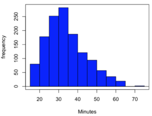
Figure 1. Histogram finishing times in minutes for 1307 runners at 2016 Banana 5K.
The task is to describe the moments for the 5K data set.
Recall: The first moment is the mean. The second moment is the variance. The third moment is skewness. And the fourth moment is kurtosis.
In R Commander, we select Statistics → Summaries → Numerical summaries…, which brings up a popup menu. First, select the variable, in this case Minutes, from the Data tab (not shown). Next, click on Statistics tab to choose options (Fig 2).
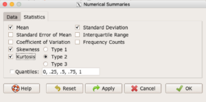
Figure 2. Rcmdr Numerical summaries Statistics tab.
For estimates of the moments, check Mean, Standard Deviation, Skewness, and Kurtosis.
Note 2: R Commander gives you the choice among three different Types of skewness and kurtosis. The default is type 2 and that’s the one you should go with. Type 1, the classical method which include the equations provided on this page, corresponding to definitions dating back to the 1940s. Type 2 is the default in R and corresponds to equations used by other professional statistics package (SAS, SPSS). Type 3 is used by other statistical packages (eg, Minitab). For large sample size, the different types will tend to agree. Caution applies to smaller data sets — the different types may disagree (Joanes and Gill 1998), although only for the third and fourth moments.
Large sample size, n = 1307
Type 1
    mean       sd  skewness    kurtosis    n
34.42999 10.31437 0.6159258 -0.01593882 1307
Type 2
    mean       sd  skewness    kurtosis    n
34.42999 10.31437 0.6166337 -0.01139521 1307
Type 3
    mean       sd skewness    kurtosis    n
34.42999 10.31437 0.615219 -0.02050335 1307
Small sample size
To test the claim about sample size and the moment statistics, draw a random sample of 30 from the larger data set. Sample without replacement
sample.banana <- data.frame(sample(banana5K$Minutes, 30, replace = FALSE))
I forgot to specify a new variable name, so R used the whole command as the variable name. I could go back and fix my function call, or simply rename the variable as follows
names(sample.banana)[c(1)] <- c("Minutes")
The random sample yielded a distribution (Fig 3).
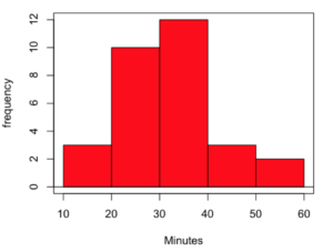
Figure 3. Histogram finishing times in minutes for random sample of 30 drawn from 1307 runners at 2016 Banana 5K.
Repeat Numerical summaries on small data set, n = 30
Type 1
    mean       sd  skewness  kurtosis  n
33.16667 10.00373 0.5538637 0.5024438 30
Type 2
    mean       sd  skewness  kurtosis  n
33.16667 10.00373 0.5834511 0.8276415 30
Type 3
    mean       sd  skewness  kurtosis  n
33.16667 10.00373 0.5264025 0.2728392 30
Conclusion: We can compare consistency of the estimators by calculating coefficient of variation. The three types of skewness estimators differed by only 1% and 5% for large and small sample size, respectively. In contrast, the three types of kurtosis estimators differed by 29% and 52% for large and small sample size, respectively.
Questions
- Explore the consistency of skewness and kurtosis estimates by calculating and comparing coefficient of variation estimates. R Commander provide a nice way to draw randomly from various defined distributions. Draw two data sets of 15 (small) and 1000 (large), from the chi-square distribution (1 degree of freedom) and a minimum of one other continuous distribution.
Example, draw random sample of 1000 from chi-square distribution. Rcmdr: Distributions → Continuous distributions → Chi-squared distribution → Sample from chi-squared distribution... (Fig 4).
Enter name for the variable, enter degrees of freedom (e.g., 1), number of samples (e.g., 1000), and number of observations (variables, columns). Leave Sample means checked under data sets.
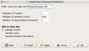
Figure 4. Screenshot Rcmdr menu: Sample from Chisquare distribution.
This results in a new data set. Get “moments” from Numerical summaries and calculate coefficient of variations. Which moments have the most consistency regardless of the kind of distribution.
- Make histograms for each of your created data sets. Describe what you see about the shape of the plotted distributions.
Quiz Chapter 6.8
Moments
Chapter 6 contents
- Introduction
- Some preliminaries
- Ratios and proportions
- Combinations and permutations
- Types of probability
- Discrete probability distributions
- Continuous distributions
- Normal distribution and the normal deviate (Z)
- Moments
- Chi-square (Χ2) distribution
- t distribution
- F distribution
- References and suggested readings