8.2 – The controversy over proper hypothesis testing

Introduction

Over the next several chapters we will introduce and develop an approach to statistical inference, which has been given the title “Null Hypothesis Significance Testing” or NHST.

In outline, NHST proceeds with

• statements of two hypotheses, a null hypothesis, H_O, and an alternate hypothesis, H_A
• calculate a test statistic comparison of the null hypothesis (assuming some characteristic of data).
• The value of the test statistic is to be compared to a critical value for the test, identified for the assumed probability distribution at associated degrees of freedom for the statistical function, and assigned Type I error rate.

We will expand on these statements later in this chapter, so stay with me here. Basically, the null hypothesis is often a statement like the responses of subjects from the treatment and control groups are the same, e.g., no treatment effect. Note that the alternate hypothesis, e.g., hypertensive patients receiving hydalazine for six weeks have lower systolic blood pressure than patients receiving a placebo (Campbell et al 2011), would be the scientific hypothesis we are most interested in. But in the Frequentist NHST approach we test the null hypothesis, not the alternate hypothesis. This framework over proper hypothesis testing is the basis of the Bayesian vs Frequentist controversy.

Consider the independent sample t-test (see Chapter 8.5 and 8.6), our first example of a parametric test.

After plugging in the sample means and the standard error for the difference between the means, we calculate t, the test statistic of the t-test. The critical value is treated as a cut-off value in the NHST approach. We have to set our Type I error rate before we start the experiment, and we have available the degrees of freedom for the test, which follows from the sample size. With these in hand, the critical value is found by looking in the t-table of probabilities (or better, use R).

For example, what is the critical value of t-test with 10 degrees of freedom and Type I error of 5%?

In Rcmdr, choose Distributions → Continuous distributions → t distribution → t quantiles…

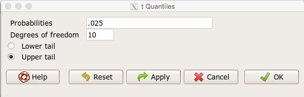
Figure 1. Screenshot t-quantiles Rcmdr

Note we want Type I equal to 5%. Since their are two tails for our test, we divide 5% by two and enter 0.025 and select the Upper tail.

R output

> qt(c(.025), df=10, lower.tail=FALSE)
[1] 2.228139

which is the same thing we would get if we look up on the t-distribution table (Fig. 2).

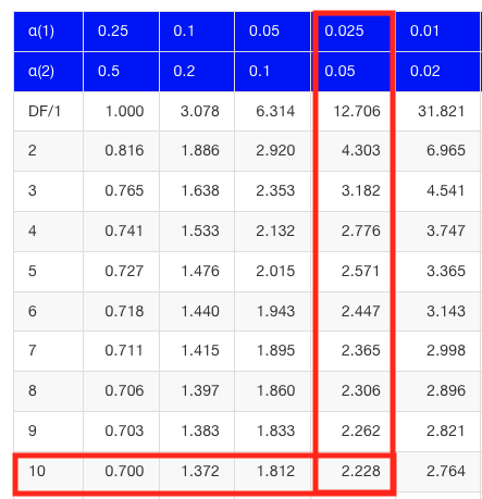
Figure 2. Screenshot of portion of t-table with highlighted (red) critical value for 10 degrees of freedom.

If the test statistic is greater than the critical value, then the conclusion is that the null hypothesis is to be provisionally rejected. We would like to conclude that the alternative hypothesis should favored as best description of the results. However, we cannot — the p-value simply tells us how likely our results would be obtained and if the null hypothesis was true. Confusingly, however, you cannot interpret the p-value as telling you the probability (how likely) that the null hypothesis is true. If however the test statistic is less than the critical value, then the conclusion is that the null hypothesis is to be provisionally accepted.

The test statistic can be assigned a probability or p-value. This p-value is judged to be large or small relative to an a priori error probability level cut off called the Type I error rate. Thus, NHST as presented in this way may be thought of as a decision path — if the test statistic is greater than the critical value, which will necessarily mean that the p value is less than the Type I error rate, then we make one type of conclusion (reject H_O). In contrast, if the test statistic is less than the critical value, which will mean that the p-value associated with the test statistic will be greater than the Type I error rate, then we conclude something else about the null hypothesis. The various terms used in this description of NHST were defined in Chapter 8.3.

Sounds confusing, but, you say, OK, what exactly is the controversy? The controversy has to do whether the probability or p-value can be interpreted as evidence for a hypothesis. In one sense, the smaller the p-value, the stronger the case to reject the null hypothesis, right? However, just because the p-value is small — the event is rare — how much evidence do we have that the null hypothesis is true? Not necessarily, and so we can only conclude that the p-value is one part of what we may need for evidence for or against a hypothesis (hint: part of the solution is to consider effect size — introduced in Chapter 9.2 — and the statistical power of the test, see Ch 11). What follows was covered by Goodman (1988) and others. Here’s the problem. Consider tossing a fair coin ten times, with the resulting trial yielding nine out of ten heads (e.g., a value of one, with tails equal to zero).

R code

set.seed(938291156)
rbinom(10,1,0.5)
[1] 1 1 1 1 1 1 0 1 1 1

While rare (binomial probability 0.0098), do we take this as evidence that the coin is not fair? By itself, the p-value provides no information about the alternative hypothesis. More about p-value follows below in sections What’s wrong with the p-value from NHST? and The real meaning and interpretation of P-values.

Statisticians have been aware of limitations of the NHST approach for years (see editorial by Wasserstein et al 2019), but only now is the message getting attention of researchers in the biosciences and other fields. In fact, the New York Times recently had a nice piece by F.D. Flam (“The Odds, Continually Updated,” 29 Sep 2014) on the controversy and the Bayesian alternative. Like most controversies there are strong voices on either side, and it can be difficult as an outsider to know which position to side with (Fig. 3).

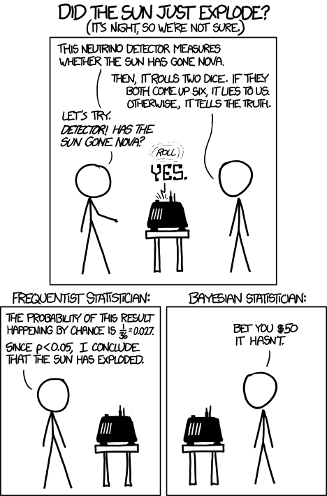
Figure 3. xkcd: Frequentists vs. Bayesians, https://xkcd.com/1132/

The short answer is — as you go forward do realize that there is a limitation to the frequentist approach and to be on the correct side of the controversy, you need to understand what you can conclude from statistical results. NHST is by far the most commonly used approached in biosciences (e.g., out of 49 research articles I checked from four randomly selected issues of 2015 PLoS Biology, 43 used NHST, 2 used a likelihood approach, none used Bayesian statistics). The NHST is also the overwhelming manner in which we teach introductory statistics courses (e.g., checking out the various MOOC courses at www.coursera.org, all of the courses related to Basic Statistics or Inferential Statistics are taught primarily from the NHST perspective). However, right from the start I want to emphasize the limits of the NHST approach.

If the purpose of science is to increase knowledge, then the NHST approach by itself is an inadequate framework at best, and in the eyes of some, worthless! Now, I think this latter sentiment is way over the top, but there is a need for us to stop before we begin, in effect, to set the ground rules for what can be interpreted from the NHST approach. The critics of NHST have a very important point, and that needs to be emphasized, but we will also defend use and teaching of this approach so that you are not left with the feeling that somehow this is a waste of time or that you are being cheated from learning the latest knowledge on the subject of statistical inference. The controversy hinges on what probability means.

P-values, statistical power, and replicability of research findings

Science, as a way of knowing how the world works, is the only approach that humans have developed that has been empirically demonstrated to work. Note how I narrowed what science is good for — if we are asking questions about the material world, then science should be your toolkit. Some (e.g., Platt 1964), may further argue that there are disciplines in science that have been more successful (e.g., molecular biology) than others (e.g., evolutionary psychology, cf discussion in Ryle 2006) at advancing our knowledge about the material world. However, to the extent research findings are based solely on statistical results there is reason to believe that many studies in fact have not recovered truth (Ioannidis 2005). In a review of genomics, it was reported that findings of gene expression differences by many microarray studies were not reproducible (Allison et al 2006). The consensus is that confidence in the findings should hold only for the most abundant gene transcripts of many microarray gene expression profiling studies, a conclusion that undercuts the perceived power of the technology to discover new causes of disease and the basis for individual differences for complex phenotypes. Note that when we write about failure of research reproducibility we are not including cases of alleged fraud (Carlson 2012 on Duke University oncogenomics case), we are instead highlighting that these kinds of studies often lack statistical power; hence, when repeated, the experiments yield different results.

Frequentist and Bayesian Probabilities

Turns out there is a lot of philosophical problems around the idea of “probability,” and three schools of thought. In the Fisherian approach to testing, the researcher devises a null hypothesis, H_O, collects the data, then computes a probability (p-value) of the result or outcome of the experiment. If the p-value is small, then this is inferred as little evidence in support of the null hypothesis. In the Frequentists’ approach, the one we are calling NHST, the researcher devises two hypotheses, the null hypothesis, H_O, and an alternate hypothesis, H_A. The results are collected from the experiment and, prior to testing, a Type I error rate (α, chance) is defined. The Type I error rate is set to some probability and refers to the chance of rejecting the null hypothesis purely due to random chance. The Frequentist then computes a p-value of result of the experiment and applies a decision criterion: If P-value greater than Type I error rate, then provisionally accept null hypothesis. In both the Fisherian and Frequentist approaches, the probability, again defined at the relative frequency of an event over time, is viewed as a physical, objective and well-defined set of values.

Bayesian approach: based on Bayes conditional probability, one identifies the prior (subjective) probability of an hypothesis, then, adjusts the prior probability (down or up) as new results come in. The adjusted probability is known as posterior probability and it is equal to the likelihood function for the problem. The posterior probability is related to the prior probability and this function can be summarized by the Bayes factor as evidence the evidence against the null hypothesis. And that’s what we want, a metric of our evidence for or against the null hypothesis.

We can calibrate the Bayesian probability to the frequentist p-value (Selke et al 2001; Goodman 2008; Held 2010; Greenland and Poole 2012). Methods to achieve this calibration vary, but the Fagan nomogram Held (2010) proposed is a good tool for us as we go forward. We can calculate our NHST p-value, but then convert the p-value to a Bayes factor by looking at the nomogram. I mention this here not as part of your to do list, but rather as a way past the controversy: the NHST p-value can be transcribed to a Bayesian conditional probability.

Likelihood

Before we move on there is one more concept to introduce, that of likelihood. We describe a model (an equation) we believe can generate the data we observe. By constructing different models with different parameters (hypotheses), you generate a statistic that yields a likelihood value. If the model fits the data, then the likelihood function has a small value. The basic idea then is to compare related, but different models to see which fits the data better. We will use this approach when comparing linear models when we introduce multiple regression models in Chapter 18.

What’s wrong with the p-value from NHST?

Well, really nothing is “wrong” with the p-value.

Where we tend to get into trouble with the p-value concept is when we try and interpret it. See below, Why is this important to me as a beginning student? The p-value is not evidence for a position, it is a statement about error rates. The p-value from NHST can be viewed as the culmination of a process that is intended to minimize the chance that the statistician makes an error.

In Bayesian terms, the p-value from NHST is the probability that we observe the data (e.g., the differences between two sample means), assuming the null hypothesis is true. If we want to interpret the p-value in terms of evidence for a proposition, then we want the conditional error probability.

Sellke et al (2001) provided a calibration of p-values and, assuming that the prior probabilities of the null hypothesis and the alternative hypothesis are equal (that is, that each have a prior probability of 0.5), by using a formula provided by them (equation 3), we can correct our NHST p-value into a probability that can be interpreted as evidence in favor of the interpretation that the null hypothesis is true. In Bayesian terms this is called the posterior probability of the null hypothesis. The formula is

where e is Euler’s number, the base of the natural logarithm (ln), and p is the p-value from the NHST. This calibration works as long as   (Sellke et al 2001).

By convention we set the Type I error at 5% (cf Cohen 1994). How strong of evidence is a p-value near 5% against the null hypothesis being true, again, under the assumption that the prior probability of the null hypothesis being true is 50%? Using the above formula I constructed a plot of the calculated conditional error probability values against p-values (Fig. 4).

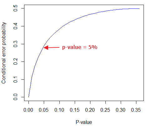
Figure 4. Conditional error probability values plotted against p-values.

As you can see, a p-value of 5% is not strong evidence at just 0.289. Not until p-values are smaller than 0.004 does the conditional error probability value dip below 0.05, suggesting strong evidence against the null hypothesis being true.

R note: For those of you keeping up with the R work, here’s the code for generating this plot. Text after “#” are comments and are not interpreted by R.

At the R prompt type each line

NHSTp = seq(0.00001,0.37,by=0.01)      #create a sequence of numbers between 0.0001 and 0.37 with a step of 0.01
CEP = (1+(-1*exp(1)*NHSTp*log(NHSTp))^-1)^-1    #equation 3 from Sellke et al 2001
plot(NHSTp,CEP,xlab="P-value", ylab="Conditional error probability",type="l",col="blue")

Why is this important to me as a beginning student?

As we go forward I will be making statements about p-values and Type I error rates and null hypotheses and even such things as false positives and false negative. We need to start to grapple with what exactly can be said by p-values in the context of statistical inference, and to recognize that we will sometimes state conclusions that cut some corners when it comes to interpreting p-values. And yet, you (and all consumers of statistics!) are expected to recognize what p-values mean. Always.

The real meaning and interpretation of P-values

This is as good of a time as any to make some clarification about the meaning of p-value and the whole inference concept. Fisher indeed came up with the concept of the p-value, but its use as a decision criterion owes to others and Fisher disagreed strongly with use of the p-value in this way (Fisher 1955; Lehmann 1993).

Here are some common p-value corner-cutting statements to avoid using (after Goodman 2008; Held 2010). P-values are sometimes interpreted, incorrectly, as

Table. Incorrect interpretations of NHST p-values

1. the probability of obtaining the observed data under the assumption of no real effect
2. an observed type-I error rate
3. the false discovery rate, i.e. the probability that a significant finding is a “false positive”
4. the (posterior) probability of the null hypothesis.

So, if p-values don’t mean any of these things, what does a p-value mean? It means that we begin by assuming that there is no effect of our treatments — the p-value is then the chance we will get as large of a result (our test statistic) and the null hypothesis is true. Note that this definition does not include a statement about evidence of the null hypothesis being true. To get evidence of “truth” we need additional tools, like the Bayes Factor and the correction of the p-value to the conditional error probability (see above). Why not dump all of the NHST and go directly to a Bayesian perspective, as some advise? The single best explanation was embedded in the assumption we made about the prior probability in order to calculate the conditional error probability. We assumed the prior probability was 50%. For many, many experiments, that is simply a guess. The truth is we generally don’t know what the prior probability is. Thus, if this assumption is incorrect, then the justification for the formula by Sellke et al (2001) is weakened, and we are no closer to establishing evidence than before. The take home message is that it is unlikely that a single experiment will provide strong evidence for the truth. Thus the message is repeat your experiments — and you already knew that!  And the Bayesians can tell us that with the addition of more and more data reduces the effect of the particular value of the prior probability on our calculation of the conditional error probability. So, that’s the key to this controversy over the p-value.

Reporting p-values

Estimated p-values can never be zero. Students may come to use software that may return p-values like “0” — I’m looking at you Google Sheets re: default results from CHISQ.TEST() — but again, this does not mean the probability of the result is zero. The software simply reports values to two significant figures and failed to round. Some journals may recommend that 0 should be replaced by p < 0.01 or even < 0.05 inequalities, but the former lacks precision and the latter over-emphasizes the 5% Type I error rate threshold, the “statistical significance” of the result. In general, report p-value to three significant figures and four digits. If a p-value is small, use scientific notation and maintain significant digits. Thus, a p-value of 0.004955794 should be reported as 0.00496 and a p-value of 0.0679 should be reported as 0.0679. Use R’s signif() function, for example p-value reported as 6.334e-05, then

signif(6.334e-05,3)
[1] 6.33e-05

Rounding and significant figures were discussed in Chapter 3.5. See Land and Altman (2015) for guidelines on reporting p-values and other statistical results.

Questions

1. Revisit Figure 1 again and consider the following hypothesis — the sun will rise tomorrow.
   • If we take the Frequentist position, what would the null hypothesis be?
   • If we take the Bayesian approach, identify the prior probability.
   • Which approach, Bayesian or Frequentist, is a better approach for testing this hypothesis?
2. Consider the pediatrician who, upon receiving a chest X-ray for a child notes the left lung has a large irregular opaque area in the lower quadrant. Based on the X-ray and other patient symptoms, the doctor diagnoses pneumonia and prescribes a broad-spectrum antibiotic. Is the doctor behaving as a Frequentist or a Bayesian?
3. With the p-value interpretations listed in the table above in hand, select an article from PLoS Biology, or any of your other favorite research journals, and read how the authors report results of significance testing. Compare the precise wording in the results section against the interpretative phrasing in the discussion section. Do the authors fall into any of the p-value corner-cutting traps?

Chapter 8 contents

• Introduction
• The null and alternative hypotheses
• The controversy over proper hypothesis testing<.span>
• Sampling distribution and hypothesis testing
• Tails of a test
• One sample t-test
• Confidence limits for the estimate of population mean
• References and suggested readings