8.3 – Sampling distribution and hypothesis testing

Introduction

Understanding the relationship between sampling distributions, probability distributions, and hypothesis testing is the crucial concept in the NHST — Null Hypothesis Significance Testing — approach to inferential statistics. is crucial, and many introductory text books are excellent here. I will add some here to their discussion, perhaps with a different approach, but the important points to take from the lecture and text are as follows.

Our motivation in conducting research often culminates in the ability (or inability) to make claims like:

1. “Total cholesterol greater than 185 mg/dl increases risk of coronary artery disease.”
2. “Average height of US men aged 20 is 70 inches (1.78 m).”
3. “Species of amphibians are disappearing at unprecedented rates.”

Lurking beneath these statements of “fact” for populations (just what IS the population for #1, for #2, and for #3?) is the understanding that not ALL members of the population were recorded.

How do we go from our sample to the population we are interested in? Put another way — How good is our sample? We’ve talked about how “biostatistics” can be generalized as sets of procedures you use to make inferences about what’s happening in populations. These procedures include:

• Have an interesting question
• Experimental design (Observational study? Experimental study?)
• Sampling from populations (Random? Haphazard?)
• Hypotheses: H_O and H_A
• Estimate parameters (characterize the population)
• Tests of hypotheses (inferences)

We have control of each of these — we choose what to study, we design experiments to test our hypotheses…We have already introduced these topics (Chapters 6 – 8).

We also obtain estimates of parameters, and inferential statistics applies to how we report our descriptive statistics (Chapter 3). Estimates of parameters like the sample mean and sample standard deviation can be assessed for accuracy and precision (e.g., confidence intervals).

Sampling distribution

Imagine drawing a sample of 30 from a population, calculating the sample mean for a variable (e.g., systolic blood pressure), then calculating a second sample mean after drawing a new sample of 30 from the same population. Repeat, accumulating one estimate of the mean, over and over again. What will be the shape of this distribution of sample means? The Central Limit Theorem states that the shape will be a normal distribution, regardless of whether or not the population distribution was normal, as long as the sample size is large (i.e., Law of Large Numbers). We alluded to this concept when we introduced discrete and continuous distributions (Chapter 6).

It’s this result from theoretical statistics that allows us to calculate the probability of an event from a sample without actually carrying out repeated sampling or measuring the entire population.

A worked example

To demonstrate the CLT we want R to help us generate many samples from a particular distribution and calculate the same statistic on each sample. We could make a for loop, but the replicate() function provides a simpler framework.  We’ll sample from the chi-square distribution. You should extend this example to other distributions on your own, see Question 5 below.

Generate x replicate samples (e.g., x = 10, 100, 1000, one million) of 30 each from chi-square distribution with one degree of freedom, test the distribution against null hypothesis (assume normal distributed, e.g., Shapiro-Wilk test, see Chapter 13.3), then make a histogram (Chapter 4.2).

x.10 <- replicate(10, {
my.mean <- rchisq(30, 1)
mean(my.mean)
})

normalityTest(~x.10, test="shapiro.test")
hist(x.10, col="orange")

Result from R

Shapiro-Wilk normality test

data: x.10
W = 0.87016, p-value = 0.1004

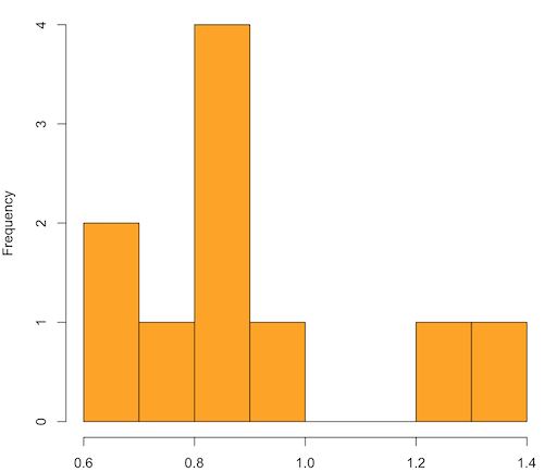
Figure 1. means of ten replicate samples drawn at random from chi-square distribution, df = 1.

Modify the code to draw 100 samples, we get

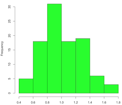
Figure 2. means of 100 replicate samples drawn at random from chi-square distribution, df = 1. Results from Shapiro-Wilks test: W = 0.97426, p-value = 0.04721

And finally, modify the code to draw one million samples, we get

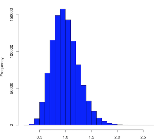
Figure 3. means of one million replicate samples drawn at random from chi-square distribution, df = 1. Normality test will fail to run, sample size of 5000 limit.

How to apply sampling distribution to hypothesis testing

First, a reminder of some definitions.

Estimate = we will always (almost) concern ourselves with how good our sample mean (such values are called estimates) is relative to the population mean, the thing we really want, but can only hope to get an estimate of.

Accuracy = how close to the true value is our measure?

Precision = how repeatable is our measure?

How can we tell if we have a good estimate? We want an estimate with an evaluation for accuracy and for precision. The sampling error provides an assessment of precision, whereas the confidence interval provides a statement of accuracy. We need an estimate of the sampling error for the statistic,

Sample standard error of the mean

We introduced sample error of the mean in section 3.4 of Chapter 3. Everything we measure can have a corresponding statement about how accurate (sampling error) is our estimate! First, we begin by asking, “how accurate is the mean that we estimate from a sample of a population?” How do we answer this? We could prove it in the mathematical sense of proof (and people have and do) OR we can use the computer to help. We’ll try this approach in a minute.

What we will show relates to the standard error of the population mean (SEM) or

, whose equation is shown below.

or equivalently, from the standard deviation we have

Note that the SEM takes the variance and divides through by the sample size. In general, then, the larger the sample size, the smaller the “error” around the mean. As we work through the different statistical tests, t-tests, analysis of variance, and related, you will notice that the test statistic is calculated as a ratio between a difference or comparison divided by some form of an error measurement. This is to remind you that “everything is variable.”

A note on standard deviation (SD) and standard error of the mean (SEM): SD estimates the variability of a sample of X_i‘s whereas SEM estimates the variability of a sample of means.

Let’s return to our thought problem and see how to demonstrate a solution. First, what is the population? Second, can we get the true population mean?

One way, a direct (but impossible?) approach would be to measure it — get all of the individuals in a population and measure them, then calculate the population mean. Then, we could compare our original sample mean against the true mean and see how close it was. This can be accomplished in some limited cases. For example, the USA conducts a census of her population every ten years, a procedure which costs billions of dollars. We can then compare samples from the different states or counties to the USA mean. And these statistics are indeed available via the census.gov website. But even the census uses sampling — individuals are randomly selected to answer more questions and from this sample trends in the population are inferred.

So, sampling from populations is the way to go for most questions we will encounter. The procedures we will use to show how a sample mean relates to the population mean are general and may be used to show how any estimate of a variable (sample mean and sample standard deviation, etc.), relates to properties of a parameter. We’ll get to the other issues, but for now, think about sample size.

Sampling from populations is necessary and inevitable, and, to a certain extent, under your control. But how many individuals do we need? The quick answer is for me to direct your attention to the equation for the SEM. Can you see in that ratio the secret to obtaining more precise estimates? There are many ways to approach this question, but let’s use the tools from last time, those based on properties of a normal distribution.

If we can view the sampling as having come from a population at least approximately normally distributed for our variable, then we can now examine empirically the effect of different sample sizes on the estimate of the mean.

A hint: variability is important!

From one population we obtain two samples, A and B. Sample sizes are

Group A, n = 9

Group B, n = 50

Assume for now that we know the true mean (μ) and standard deviation (σ) for the population. Note. This is one of the points of why we use computer simulation so much to teach statistics — it allows us to specify what the truth is, then see how our statistical tools work or how our assumptions affect our statistically based conclusions.

μ = 47.0 mm
σ = 12.0 mm

Confidence intervals

Reliability is another word for precision. We define a confidence interval as a statistic to report the reliability of our estimated statistic. We introduced confidence interval in section 3.4 of Chapter 3. At least in principle, confidence intervals can be calculated for all statistics (mean, variance, etc.,) and for all data types. Confidence intervals define a lower limit, L, and an upper limit, U, and that you are making a statement that you are “95% certain that the true value (parameter value) is between these two limits.

We previously reported how to calculate an approximate confidence intervals for proportions and for NNT; simply multiple standard error estimate by 2. Here we introduce an improved approximate calculation of the 95% confidence interval for the sample mean

where Z is something you would look up from the table of the normal distribution. For a 95% confidence interval, 100% – 95% = 5% and divide 5% by two: the lower limit corresponds to 2.5% and the upper limit corresponds to 2.5% on our normal distribution. We look up the table and we find that Z for 0.025 is 1.96 and that is the value we would plug into our equation above. For large sample sizes, you can get a pretty decent estimate of the confidence interval by replacing 1.96 with “2.”

Questions

1. What is the probability of having a sample mean greater than 50 (mean > 50) for a sample of n = 9 ?

We’ll use a slight modification of the Z-score equation we introduced in Chapter 6.6 — the modification here is that previously we referred to the distribution of Xi‘s and how likely a particular observation would be. Instead, we can use the Z score with the standard normal distribution (aka Z-distribution), approach to solving how likely an estimated sample mean is given the population parameters μ and σ. Recall the Z score

We have everything we need except the SEM, which we can calculate by dividing the standard deviation by squared root of sample size.

For

, σ = 12.0 (given above), and μ = 47, n = 9, plug in the values:

Therefore, after applying the equation for Z score, Z = 0.75. This corresponds to how far away from the standard mean of zero.

Look up Z = 0.75 from the table of normal distribution. The answer is 0.22663, which corresponds to that Z is EQUAL to or GREATER than 0.75, which is what we wanted. Translated, this implies that, given the level of variability in the sample, 22.66% of your sample means would be greater than 50! We write: P(X > 50.0) = P (Z > 0.75) = 0.2266

Some care needs to be taken when reading these tables — make sure you understand how the direction (less than, greater than) away from the mean is tabulated.

2. Instead of greater, how would you get the probability less than 50?

Total area under the curve is 1 (100%), so subtract 1 from 0.22663 = 0.7734.

I recommend that you do these by hand first, then check your answers. You’ll need to be able to do this for exams.

Here’s how to use Rcmdr to do these kind of problems.

Rcmdr: Distributions → Continuous distributions → Normal distribution → Normal probabilities …

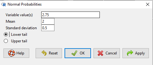
Figure 1. Screenshot Rcmdr menu to get normal probability

Here’s the answer from Rcmdr

pnorm(c(50), mean=47, sd=12, lower.tail=TRUE)

[1] 0.5987063

3. Now, try a larger sample size. For N = 50, what is the probability of having a sample mean greater than 50 (mean > 50)?

, μ = 47, σ = 12, n = 50 and

Therefore, after applying the equation for Z score, Z = 1.768. Look up Z = 1.768 (Normal table, subtract answer from 1) and we get 0.0384.

Or 3.84% of your sample means would be greater than 50! We write: P(X > 50.0) = P (Z > 1.768) = 0.0384.

Said another way: If you have a sample size of 50 (N = 50 ) and you obtain a mean greater than 50 then there is only a 3.84% chance that the TRUE MEAN IS 47.

4. What happens if the variability is smaller? Chance σ from 12 to 6 then repeat questions 1 and 4.

5. Repeat the demonstration of Central Limit Theorem and Law of Large Numbers for discrete  distributions

1. binomial distribution. Replace rchisq() with rbinom(n, size, prob) in the replicate() function example. See Chapter 6.5
2. poisson distribution. Replace rchisq() with rpois(n, lambda) in the replicate() function example. See Chapter 6.5

Chapter 8 contents

• Introduction
• The null and alternative hypotheses
• The controversy over proper hypothesis testing
• Sampling distribution and hypothesis testing
• Tails of a test
• One sample t-test
• Confidence limits for the estimate of population mean
• References and suggested readings