12.7 – Many tests one model
Introduction
In our introduction to parametric tests we so far have covered one and two sample t-tests and now the multiple sample or one-way analysis of variance (ANOVA). In subsequent sections we will cover additional tests, each with their own name. It is time to let you in on a little secret. All of these tests, t-tests, ANOVA, and linear and multiple regression we will work on later in the book belong to one family of statistical models. That model is called the general Linear Model (LM), not to be confused with the Generalized Linear Model (GLM) (Burton et al 1998; Guisan et al 2002). This greatly simplifies our approach to learning how to implement statistical tests in R (or other statistical programs) — you only need to learn one approach: the general Linear Model (LM) function lm().
Brief overview of linear models
With the inventions of correlation, linear regression, t-tests, and analysis of variance in the period between 1890 and 1920, subsequent work led to the realization that these tests (and many others!) were special cases of a general model, the general linear model, or LM. The LM itself is a special case of the generalized linear model, or GLM; among the differences between LM and GLM, in LM, the dependent variable is ratio scale and errors in the response (dependent) variable(s) are assumed to come from a Gaussian (normal) distribution. In contrast, for GLM, the response variable may be categorical or continuous, and error distributions other than normal (Gaussian), may be applied. The GLM user must specify both the error distribution family (eg, Gaussian) and the link function, which specifies the relationship among the response and predictor variables. While we will use the GLM functions when we attempt to model growth functions and calculate EC50 in dose-response problems, we will not cover GLM this semester.
The general Linear Model, LM
In matrix form, the LM can be written as

where  is a matrix of response variables predicted by independent variables contained in matrix
  and weighted by linear coefficients in the vector b. Basically, all of the predictor variables are combined to produce a single linear predictor
  . By adding an error component we have the complete linear model.

In the linear model, the error distribution is assumed to be normally distributed, or “Gaussian.”
R code
The bad news is that LM in R (and in any statistical package, actually) is a fairly involved set of commands; the good news is that once you understand how to use this command, and can work with the Options, you will be able to conduct virtually all of the tests we will use this semester, from two-sample t-tests to multiple linear regression. In the end, all you need is the one Rcmdr command to perform all of these tests.
We begin with a data set, ohia.ch12. Scroll down this page or click here to get the R code.
I found a nice report on a common garden experiment with o`hia (Corn and Hiesey 1973). O`hia (Metrosideros polymorpha) is an endemic, but wide-spread tree in the Hawaiian islands (Fig 1). O`hia exhibits pronounced intraspecific variation: individuals differ from each other. O`hia grows over wide range of environments, from low elevations along the ocean right up the sides of the volcanoes, and takes on many different growth forms, from shrubs to trees. Substantial areas of o`hia trees on the Big Island are dying, attributed to two exotic fungal species of the genus Ceratocystis (Asner et al., 2018).

Figure 1. O’hia, Metrosideros polymorpha. Public domain image from Wikipedia.
The Biology. Individuals from distinct populations may differ because the populations differ genetically, or because the environments differ, or, and this is more realistic, both. Phenotypic plasticity is the ability of one genotype to produce more than one phenotype when exposed to different environments. Environmental differences are inevitable when populations are from different geographic areas. Thus, in population comparisons, genetic and environmental differences are confounded. A common garden experiment is a crucial genetic experiment to separate variation in phenotypes, P, among populations into causal genetic or environmental components.
If you recall from your genetics course, 
where G stands for genetic (alleles) differences among individuals and E stands for environmental differences among individuals. In brief, the common garden experiment begins with individuals from the different populations are brought to the same location to control environmental differences. If the individuals sampled from the populations continue to differ despite the common environment, then the original differences between the populations must have a genetic basis, although the actual genetic scenario may be complicated (the short answer is that if “genotype by environment interaction exists, then results from a common garden experiment cannot be generalized back to the natural populations/locations — this will make more sense when we talk about two-way ANOVA). For more about common garden experiments, see de Villemereuil et al (2016). Nuismer and Gandon (2008) discuss statistical aspects of the common garden approach to studying local adaptation of populations and the more powerful “reciprocal translocation” experimental design.
Managing data for linear models
First, your data must be stacked in the worksheet. That means one column is for group labels (independent variable), the other column is for the response (dependent) variable.
If you have not already downloaded the data set, ohia.ch12, do so now. Scroll down this page or click here to get the R code.
Confirm that the worksheet is stacked. If it is not, then you would rearrange your data set using Rcmdr: Data → Active data set → Stack variables in data set…
The data set contains one factor, “Site” with three levels (M-1, 2, 3). M stands for Maui, and collection sites were noted in Figure 2 of Corn and Hiesey (1973). Once the dataset is in Rcmdr, click on View to see the data (Fig 2). There are two response variables, Height (shown in red below) and Width (shown in blue below).
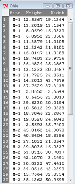
Figure 2. The o`hia dataset as viewed in R Commander.
The data are from Table 5 of Corn and Hiesey 1973. (I simulated data based on their mean/SD reported in Table 5). This was a very cool experiment: they collected o`hia seeds from three elevations on Maui, then grew the seeds in a common garden in Honolulu. Thus, the researchers controlled the environment; what varied, then were the genotypes.
As always, you should look at the data. Box plots are good to compare central tendency (Fig 3).
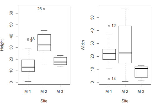
Figure 3. Box plots of growth responses of o`hia seedlings collected from three Maui sites, M-1 (elevation 750 ft), M-2 (elevation 1100 ft), and M-3 (elevation 6600 ft). Data adapted from Table 5 of Corn and Hiersey 1973.
R code to make Figure 4 plots
par(mfrow=c(1,2))
Boxplot(Height ~ Site, data = ohia, id = list(method = "y"))
Boxplot(Width ~ Site, data = ohia, id = list(method = "y"))
This dataset would typically be described as a one-way ANOVA problem. There was one treatment variable (population source) with three levels (M-1, M-2, M-3). From Rcmdr we select the one-way ANOVA: Statistics → Means → One-way ANOVA… and after selecting the Groups (from the Site variable) and the Response variable (eg, Height), we have
AnovaModel.1 <- aov(Height ~ Site, data = ohia.ch12)
summary(AnovaModel.1)
           Df Sum Sq   Mean Sq  F value          Pr(>F)
Site        2   4070    2034.8    22.63 0.000000131 ***
Residuals  47   4227      89.9
---
Signif. codes: 0 '***' 0.001 '**' 0.01 '*' 0.05 '.' 0.1 ' ' 1
Let us proceed to test the null hypothesis (what was it???) using instead the lm() function. Four steps in all.
Step 1. Rcmdr: Statistics → Fit models → Linear model … (Fig 4).
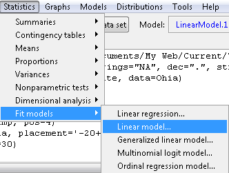
Figure 4. R Commander, select to fit a Linear model.
Step 2. The pop up menu below (Fig 5) follows.
First, What is our response (dependent) variable? What is our predictor (independent) variable? We then input our model. In this case, with only the one predictor variable, Sites, our model formula is simple to enter (Fig 5): Height ~ Site.
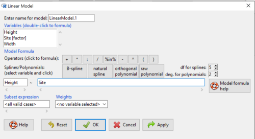
Figure 5. Input linear model formula, Height ~ Site.
Step 3. Click OK to carry out the command.
Here is the R output and the statistical results from the application of the linear model.
LinearModel.1 <- lm(Height ~ Site, data=ohia.ch12)
summary(LinearModel.1)

Call:
lm(formula = Height ~ Site, data = ohia.ch12)

Residuals:
    Min     1Q   Median     3Q     Max
-18.808 -4.761   -1.755  4.758  29.257

Coefficients:
             Estimate  Std. Error  t value      Pr(>|t|)
(Intercept)    15.314       2.121    7.222 0.00000000377 ***
Site[T.M-2]    19.261       2.999    6.423 0.00000006153 ***
Site[T.M-3]     2.924       3.673    0.796          0.43
---
Signif. codes:  0 '***' 0.001 '**' 0.01 '*' 0.05 '.' 0.1 ' ' 1
Residual standard error: 9.483 on 47 degrees of freedom
Multiple R-squared:  0.4905,	Adjusted R-squared:  0.4688
F-statistic: 22.63 on 2 and 47 DF,  p-value: 0.0000001311
End R output
The linear model has produced a series of estimates of coefficients for the linear model, statistical tests of the significance of each component of the model, and the coefficient of determination, R2, which is a descriptive statistic of how well model fits the data. Instead of our single factor variable for Source Population like in ANOVA we have a series of what are called dummy variables or contrasts between the populations. Thus, there is a coefficient for the difference between M-1 and M-2. “Site[T.M-2]” in the output, between M-1 and M-3, and between M-2 and M-3.
Note 1: Brief description of linear model output; these will be discussed fuller in Chapter 17 and Chapter 18. The residual standard error is a measure of how well a model fits the data. The Adjusted R-squared is calculated by dividing the residual mean square error by the total mean square error. The result is then subtracted from 1.
It also produced our first statistic that assesses how well the model fits the data called the coefficient of determination, R2. An of of 1.0 would indicate that all variation in the data set can be explained by the predictor variable(s) in the model with no residual error remaining. Our value of 49% indicates that nearly 50% of the variation in height of the seedlings grown under common environments are due to the source population (= genetics).
Step 4. But we are not quite there — we want the traditional ANOVA results (recall the ANOVA table).
To get the ANOVA Table we have to ask Rcmdr (and therefore R) to give us this. Select
Rcmdr: Models → Hypothesis tests → ANOVA table … (Fig 6).
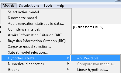
Figure 6. To retrieve an ANOVA table, select Models, Hypothesis tests, then ANOVA table…
Here’s the type of tests for the ANOVA table, select the default (Fig 7).
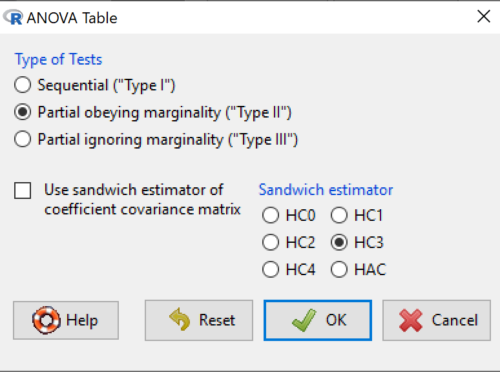
Figure 7. Options for types of tests.
Now, in the future when we work with more complicated experimental designs, we will also need to tell R how to conduct the test. For now, we will accept the default Type II type of test and ignore sandwich estimators. You should confirm that for a one-way ANOVA, Type I and Type II choices give you the same results.
The reason they do is because there is only one factor — when there are more than one factors, and if one or both of the factors are random effects, then Type I, II, and III will give you different answers. We will discuss this more as needed, but see the note below about default choices.
Note 2: Marginal or partial effects are slopes (or first derivatives): they quantify the change in one variable given change in one or more independent variables. Type I tests are sequential: sums of squares are calculated in the order the predictor variables are entered into the model. Type II tests the sums of squares are calculated after adjusting for some of the variables in the model. Type III, every sum of square calculation is adjusted for all other variables in the model. Sandwich estimator refers to algorithms for calculating the structure of errors or residuals remaining after the predictor variables are fitted to the data. The assumption for ordinary least square estimation (See Chapter 17) is that errors across the predictors are equal, ie, equal variances assumption. HC refers to “heteroscedasticity consistent” (Hayes and Chai 2007), which infers fitting of a model does not assume equal error variance across all observations.
By default, Rcmdr makes Type II. In most of the situations we will find ourselves this semester, this is the correct choice.
Below is the output from the ANOVA table request. Confirm that the information is identical to the output from the call to aov() function.
Anova(LinearModel.1, type = "II")
Anova Table (Type II tests)
Response: Height
          Sum Sq  Df   F value        Pr(>F)
Site      4069.7   2    22.626  0.0000001311 ***
Residuals 4226.9  47
---
Signif. codes: 0 '***' 0.001 '**' 0.01 '*' 0.05 '.' 0.1 ' ' 1
And the other stuff we got from the linear model command? Ignore for now but make note that this is a hint that regression and ANOVA are special cases of the same model, the linear model.
We do have some more work to do with ANOVA, but this is a good start.
Why use the linear model approach?
Chief among the reasons to use the lm() approach is to emphasize that a model approach is in use. One purpose of developing a model is to provide a formula to predict new values. Prediction from linear models is more fully developed in Chapter 17 and Chapter 18, but for now, we introduce the predict() function with our O`hia example.
myModel <- predict(LinearModel.1, interval = "confidence")
head(myModel, 3)    #print out first 3 rows
#Add the output to the data set
ohiaPred <- data.frame(ohia,myModel)
with(ohiaPred, tapply(fit, list(Site), mean, na.rm = TRUE))   #print out predicted values for the three sites
Output from R
myModel <- predict(LinearModel.1, interval = "confidence")
head(myModel, 3)
       fit      lwr      upr
1 15.31374 11.04775 19.57974
2 15.31374 11.04775 19.57974
3 15.31374 11.04775 19.57974
with(myModel, tapply(fit, list(Site), mean, na.rm = TRUE))
     M-1      M-2      M-3
15.31374 34.57474 18.23796
Questions
1. Revisit ANOVA problems in homework and questions from early parts of this chapter and apply lm() followed by Hypothesis testing (Rcmdr: Models → Hypothesis tests → ANOVA table) approach instead of one-way ANOVA command. Compare results using lm() to results from One-way ANOVA and other ANOVA problems.
Quiz Chapter 12.7
Many tests one model
Data set and R code used in this page
Corn and Hiesey (1973)
| Site | Height | Width |
|---|---|---|
| M-1 | 12.5567 | 19.1264 |
| M-1 | 13.2019 | 13.1547 |
| M-1 | 8.0699 | 16.032 |
| M-1 | 6.0952 | 22.8586 |
| M-1 | 11.3879 | 11.0105 |
| M-1 | 12.2242 | 21.8102 |
| M-1 | 16.0147 | 11.0488 |
| M-1 | 19.7403 | 25.9756 |
| M-1 | 36.4824 | 25.2867 |
| M-1 | 13.1233 | 20.0487 |
| M-1 | 21.7725 | 24.8511 |
| M-1 | 14.2013 | 43.7679 |
| M-1 | 37.7629 | 37.3438 |
| M-1 | 2.8652 | 2.5549 |
| M-1 | 0.6456 | 22.8013 |
| M-1 | 29.623 | 20.0194 |
| M-1 | 10.5812 | 29.0328 |
| M-1 | 18.3046 | 22.2867 |
| M-1 | 19.0528 | 24.684 |
| M-1 | 2.5693 | 35.74 |
| M-2 | 45.0162 | 14.3878 |
| M-2 | 40.8404 | 18.8396 |
| M-2 | 27.1032 | 21.0547 |
| M-2 | 29.8036 | 16.9327 |
| M-2 | 63.8316 | 30.7037 |
| M-2 | 42.107 | 3.2491 |
| M-2 | 30.0322 | 47.4412 |
| M-2 | 34.0516 | 42.239 |
| M-2 | 15.7664 | 32.8354 |
| M-2 | 35.1262 | 50.9698 |
| M-2 | 43.6988 | 19.3897 |
| M-2 | 26.7585 | 13.8168 |
| M-2 | 36.7895 | 0.5817 |
| M-2 | 30.9458 | 53.7757 |
| M-2 | 26.8465 | 15.4137 |
| M-2 | 40.3883 | 9.2161 |
| M-2 | 30.6555 | 56.8456 |
| M-2 | 19.9736 | 44.9411 |
| M-2 | 27.676 | 36.8543 |
| M-2 | 44.084 | 24.3396 |
| M-3 | 15.2646 | 11.4999 |
| M-3 | 19.6745 | 9.7757 |
| M-3 | 23.275 | 12.7825 |
| M-3 | 16.1161 | 2.4065 |
| M-3 | 16.8393 | 1.1253 |
| M-3 | 23.107 | 3.7349 |
| M-3 | 21.5322 | 6.9725 |
| M-3 | 13.4191 | 12.2867 |
| M-3 | 14.7273 | 11.4841 |
| M-3 | 18.4245 | 11.9078 |