6.3 – Combinations and permutations
Introduction
In statistical inference, an important foundational skill is to be able to count the possible outcomes of an experiment — the sample space. For example, when drawing on a sample of individuals for study from specific groups (strata) of a population, combinations may be calculated; where it is unwarranted to assume a particular theoretical probability distribution applies, permutation tests create a reference distribution by calculating all possible values of a test statistic under rearrangements of the observed data.
The simplest place to begin with probability is to define an event — an event is an outcome — a “Heads” from a toss of coin, or the chance that the next card dealt is an ace in a game of Blackjack. In these simple cases we can enumerate how likely these events are given a number of chances or trials. For example, if the coin is tossed once, then the coin will either land “Heads” or “Tails” (Fig 1).
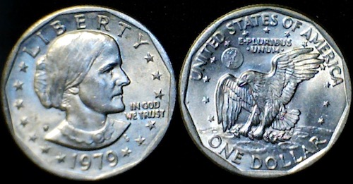
Figure 1. Heads (left) and Tails (right) of a USA Susan B. Anthony dollar.
We can then ask what is the likelihood of ten “Heads” in ten tosses of a fair coin?
And this gets us to some basic rules of probability:
- if successive events are independent, then we multiply the probability
- if events are not independent, then the probability adds
- do we sample without replacement, i.e., an object can only be used once?
- do we sample with replacement, i.e., an object gets placed “back in the deck” and can be used again and again
Combinations and Permutations
Both combinations and permutations pertain to how samples are selected from a population. Combinations are used if the events or objects of the sample are all of the same kind, whereas for permutations, it is implied that the events or objects are not all of the same kind.
Figure 2. A combination lock
Combinations ignore the order of the events; permutations are ordered combinations. For replacement, the formula for permutations is simply 
In the case of the ten “Heads,” in ten successive trials, the probability is  “ten-times” or
  = 0.0009766 (in R, just type
 0.5^10 or (1/2)^10 at the R prompt).
Examples of permutations in biology include,
Given the four nucleotide bases of DNA, adenine (A), cytosine (C), guanine (G), and thymine (T), how many codons are possible?

where the three (3) refers to the codon, three nucleotide genetic code. Codons are trinucleotide sequences of DNA or RNA that correspond to a specific amino acid. For transcription initiation of a protein-coding gene, a key sequence must be present in the promoter region of the gene. In Archaea and Eukaryotes, that sequence is called the TATA box. How often do we expect to find by chance the heptamer (ie, seven bases) TATA box sequence in the human genome?
Note 1: The consensus TATA box sequence, TATAWAW (W can be either Adenine or Thymine, per Standard IUB/IUPAC nucleic acid code). The TATA box is the binding site for transcription factors, particularly the TATA binding protein.

Thus, we would expect at random to find TATA box sequences every 16,384 bases along the genome. For the human genome of 3.3 billion bases then we would expect at random more than 200,000 TATA box consensus sequences.
Another way to put this is to ask how many combinations of ten tosses gets us ten “Heads” then weigh this against all possible outcomes of tossing a coin ten times — how many times do we get zero Heads? Two “Heads”? And so on. This introduces the combinatorial.

where n is the number of choices (the list of events) and r is how many times you choose or trials. The exclamation point is called the factorial. The factorial instructs you to multiply the number over and over again, “down to one.” For example, if the number is 10, then

In R, just type factorial(10) at the R prompt.
factorial(10)
[1] 3628800
An example
Consider an extrasensory perception, ESP, experiment. We place photocopies of two kinds of cards, “Queen” and “King,” into ten envelopes, one card per envelope (Fig 2). Thus, an envelope either contains a “Queen” or a “King.”
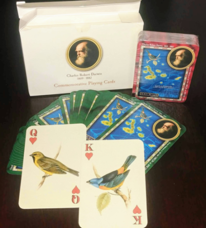
Figure 2. Playing cards with images commemorating 150th anniversary of Charles Darwin’s Origin of Species. (Design John R. C. White, Master of the Worshipful Company of Makers of Playing Cards 2008 to 2009.)
We shuffle the envelopes containing the cards and volunteers guess the contents of the envelopes, one at a time. We score the correct choices after all envelopes had been guessed. (It’s really hard to set these kinds of experiments up to rule out subtle cues and other kinds of experimental error! Diaconis 1978, Pigliucci 2010, pp. 77 – 83.) By chance alone we would expect 50% correct (e.g., one way to game the system would have been for the volunteer simply to guess “Queen” every time; since we had placed five “Queen” cards the volunteer would end up being right 50%).
What are the possible combinations?
Let’s start with one correct; the volunteer could be right by guessing the first one correctly, then getting the next nine wrong, or equivalently, the first choice was wrong, but the second was correct followed by eight incorrect choices, and so on.
We need math!
Let n = 10 and r = 1
Using the formula above we have

or ten ways to get one out of ten correct. This is the number of combinations without replacement.
In R, we can use the function choose(), included in the base install of R. At the R prompt type
choose(10,1)
and R returns
[1] 10
For permutations, use choose(n,k)*factorial(k).
To get permutations for larger sets, you’ll need to write a function or take advantage of functions written by others and available in packages for R. See gtools package, which contains programming tools for R. There are several packages that can be used to expand capabilities of working with permutations and combinations. For example, install a package and library called combinat and then run the combn() function, together with the dim() function, which will return
dim(combn(10,1))[2]
[1] 10
R explained
In the combn() the “10” is the total number of envelopes and the “1” is how many correct guesses. We also used the dim() function to give us the size of the result. The dim() function returns two numbers, the number of rows and the number of columns — combn() returns a matrix and so dim() saves you the trouble of counting the outcomes — the “[2]” tells R to return the total number of columns in the matrix created by combn(). Here’s the output from combn() , but without the dim() function
combn(10,1)
     [,1] [,2] [,3] [,4] [,5] [,6] [,7] [,8] [,9] [,10]
[1,]    1    2    3    4    5    6    7    8    9    10
in order, we see that there is one case where the success came the first time [1,1], another case where success came on the second try [1,2] and so on.
We can write a simple function to return the combinations
for (many in seq(0, 10, by = 1)){
    print(choose(10, many))
}
an inelegant function, but it works well enough, returning
[1] 1
[1] 10
[1] 45
[1] 120
[1] 210
[1] 252
[1] 210
[1] 120
[1] 45
[1] 10
[1] 1
Note that there’s only one way to get zero correct, only one way to get all ten correct.
For completion, what would be the permutations? Use the permn() function (same combinat library) along with length() function to get the number of permutations
length(permn(10))
[1] 3628800
Continue the example
Back to our ESP problem. If we continue with the formula, how many ways to get two correct? Three correct? And so on, we can show the results in a bar graph (Fig. 3).
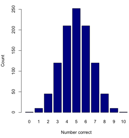
Figure 3. Bar chart of the combinations of correct guesses out of 10 attempts (graph was presented in Chapter 4.1).
The graph in Figure 3 was made in R
Combos <- seq(0,10, by=1)
HowMany <- c(1,10,45,120,210,252,210,120,45,10,1)
barplot(HowMany, names.arg = Combos, xlab = "Number correct", ylab = "Count",col = "darkblue")
If you recall, we had two students score eight out of ten. Is this evidence of “ESP?” It certainly seems pretty good, but how rare is this to score 8 out of 10? The total number of outcomes was

Eight out of ten could be achieved in 45 different ways, so

So, eight out of ten is pretty unlikely! Is it evidence for ESP powers in our Biostatistics class? In fact, at the traditional Type I error rate of 5% used in biology and other sciences to evaluate inferences from statistical tests (See Chapter 8), we would say that this observation was statistically significant. Given that this would be an extraordinary claim, this should give you an important clue that statistical significance is not the same thing as evidence for the claim of ESP.
Note 2: This is a good example where frequentist approach may not be the best approach — the Bayesian prior probability for ESP is vanishingly low. See O’Hagan (2006) for a similar ESP problem worked from a Bayesian perspective.
In other words, Is our result biologically significant? Probably not, but I’ll keep my eyes on you, just in case.
Conclusions
Combinations or permutations?
Combinations refers to groups of n things taken k times without repetition. Note that order does not matter, just the combination of things. Permutations, on the other hand, specifically relate the number of ways a particular arrangement can show up.
Questions
- Calculate the combinations, from zero correct to ten correct, from our ESP experiment, i.e., confirm the numbers reported in Figure 3.
- Consider our ESP tests based on guessing cards. Let’s say that one subject repeatedly reports correct guesses at a rate greater than expected by chance. Why or why not should we view this as evidence the person may have extrasensory perception?
- Return to our TATA box example. The number of protein-coding genes in the human genome is presently estimated to be 20,620 (NCBI August 2025). Given that each gene has one promoter sequence, what proportion of TATA boxes are not associated with protein-coding genes?
- Assuming a standard 52-card deck, how many possible 5-card poker hands — the set of cards a player holds during a round of play — are there?
Quiz Chapter 6.3
Combinations and permutations
Chapter 6 contents
- Introduction
- Some preliminaries
- Ratios and probabilities
- Combinations and permutations
- Types of probability
- Discrete probability distributions
- Continuous distributions
- Normal distribution and the normal deviate (Z)
- Moments
- Chi-square distribution
- t distribution
- F distribution
- References and suggested readings