14.8 – More on the linear model in Rcmdr
Introduction
During the last lectures, we could have used the Two-Way ANOVA command in R or Rcmdr
R code: How to analyze multifactorial ANOVA problems
Rcmdr: Statistics → Means → Multiway ANOVA
To analyze our two factor data sets. As long as the design meets the following conditions, by all means use this command because it is simple and precisely correct.
- Both factors are fixed, not random.
- Each level of first factor is crossed with each level of the second factor.
- No missing data (the design is fully replicated and balanced).
If any of the three points do not fit your two-way design, then you’ll need a different, more general and powerful ANOVA procedure in R and Rcmdr to analyze these types of designs. You’ll need the lm() function (Fig. 1).
Rcmdr: Statistics → Fit models → Linear model…
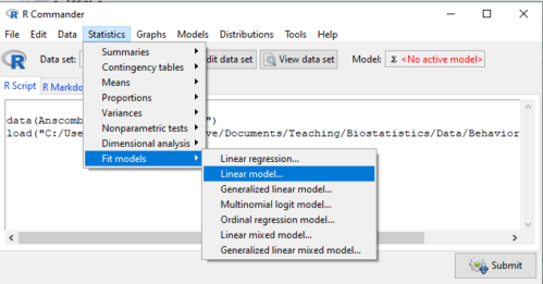
Figure 1. Linear model menu in Rcmdr, version 2.7.0
Some R basics with the lm() function, the general linear model.

Response  is specified by linear predictor(s), either factors or covariates (ratio-scale predictor variables). We communicate to R what the model is by using operators. The four more commonly used operators are
 the basic way to include the model terms, i.e., the mode predictors
 which is interpreted as the interaction of all the variables and the factors in the term
 is interpreted as factor crossing
Not shown, but  indicates the term on the left is nested within the term on the right.
A few examples: we’ll have three factors, A, B, and C. For our one-way ANOVA, the model specification would be

For our crossed, balanced two-way ANOVA, the model specification would be

or equivalently

And for our block ANOVA problem?
Click here to get entire List of model commands in R.
How would we analyze our snake experiment?
Table 1. The snake data set
| Snake | Source | flick |
| 1 | dH2O | 3 |
| 2 | dH2O | 0 |
| 3 | dH2O | 0 |
| 4 | dH2O | 5 |
| 5 | dH2O | 1 |
| 6 | dH2O | 2 |
| 1 | fish | 6 |
| 2 | fish | 22 |
| 3 | fish | 12 |
| 4 | fish | 24 |
| 5 | fish | 16 |
| 6 | fish | 16 |
| 1 | worm | 6 |
| 2 | worm | 22 |
| 3 | worm | 12 |
| 4 | worm | 24 |
| 5 | worm | 16 |
| 6 | worm | 16 |
We have two factors, but one factor is a Block (repeated measures on individuals). We need to tell R and Rcmdr what our model is. We’ll return to talk about models next time, a very important topic!! For now, think of a model as adding the independent variables together to predict the response variable.
In our Snake example, it’s a two-way ANOVA, but one factor is individual snake, the other is a treatment, and we have repeat measures, so there cannot be an interaction.
We tell R and Rcmdr which columns contain the Response, and under Model, we enter the columns with the two factors.
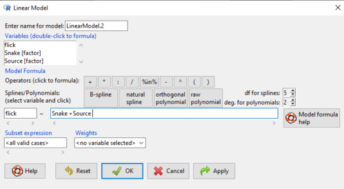
Figure 2. Menu of linear model with repeat measures model, Rcmdr, version 2.7.0.
You must also tell R and Rcmdr which factors in the model (if any) are random to get the correct F statistics. Almost without exception, blocking factors are always treated as Random
The output looks like this (see below). More complicated, true (which means more information!), but things marked in red we’ve seen before.
LinearModel.2 <- lm(flick ~ Snake +Source, data=L16SnakeTaste)

summary(LinearModel.2)

Call:
lm(formula = flick ~ Snake + Source, data = L16SnakeTaste)

Residuals:
Min 1Q Median 3Q Max
-5.2222 -0.7222 0.0278 1.5694 7.4444

Coefficients:
             Estimate Std. Error t value Pr(>|t|)
(Intercept)    -4.444      2.523  -1.762 0.10862
Snake[T.2]      9.667      3.090   3.128 0.01072 *
Snake[T.3]      3.000      3.090   0.971 0.35451
Snake[T.4]     12.667      3.090   4.099 0.00215 **
Snake[T.5]      6.000      3.090   1.942 0.08085 .
Snake[T.6]      6.333      3.090   2.050 0.06755 .
Source[T.fish] 14.167      2.185   6.484 0.0000704 ***
Source[T.worm] 14.167      2.185   6.484 0.0000704 ***
---
Signif. codes: 0 '***' 0.001 '**' 0.01 '*' 0.05 '.' 0.1 ' ' 1

Residual standard error: 3.784 on 10 degrees of freedom
Multiple R-squared: 0.8858, Adjusted R-squared: 0.8058
F-statistic: 11.08 on 7 and 10 DF, p-value: 0.0005337
Contrast coding
When a factor (categorical variable) is used in a linear model (lm() or aov()), R must convert the factor into one or more numeric predictor variables. Contrast coding tells us how to represent the factor in the model, how to interpret the coefficients associated with the factor, how the hypothesis tests of the coefficients are handled, and whether or not Type III sums of squares tests are valid. R can handle contrast coding in a couple of ways, either as a dummy contrast (each group if the factor is contrasted to a baseline) or effects coding, where group means are compared to the grand mean. The command summary(lm()) reports contrast coding that was used in the linear model. Every kind of contrast leads to the same fitted values and same overall F-test, but coefficient estimates and t-tests change.
Note 1: Type I sums of squares tests are affected by the order of the predictors in the model, not by type of contrast coding used. R Commander defaults to Type II tests, which are generally unaffected by coding contrasts used. In contrast, Type III tests are affected by the type of coding contrasts used — Type III tests require sum-to-zero (effects) contrasts.
For the ANOVA table, we call up the command via
Rcmdr: Models → Hypothesis tests → ANOVA table… (Fig. 3).
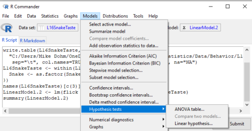
Figure 3. Rcmdr: Models → Hypothesis tests → ANOVA table… Rcmdr, version 2.7.0
Confirm that the model object is active (in this case, the object was LinearModel.2), accept the defaults about types of tests and marginality, and submit OK. The output is
Anova(LinearModel.2, type="II")
Anova Table (Type II tests)

Response: flick
          Sum Sq Df F value Pr(>F)
Snake     307.61  5  4.2956 0.02396 *
Source    802.78  2 28.0256 0.00007954 ***
Residuals 143.22 10
---
Signif. codes: 0 '***' 0.001 '**' 0.01 '*' 0.05 '.' 0.1 ' ' 1
End R output
You do not need to know all of the output; all of that output is there for a reason, of course, but for now, here’s what R and Rcmdr has to say (from the help menu):
The sequential sums of squares is the added sums of squares given that prior terms are in the model. These values depend upon the model order. The adjusted sums of squares are the sums of squares given that all other terms are in the model. These values do not depend upon the model order.
You should try our snake example again, but this time, remove the tongue flick response to the dH2O for the first snake — a missing value. (just type into the cell NA).
How would you use GLM to analyze a simple two-way ANOVA, a fully crossed, fully replicated (“balanced”) design? We could use the Two-way ANOVA command in R and Rcmdr, or we could use lm(). Try it with the data set from random vs nonrandom lecture.
Another example
Below, you see how the model is entered. To let R know that I wish R and Rcmdr to test the interaction, I need to add a Model term for that source of variation. I accomplish this by typing “Diet*Drug” (without the quotes).

Figure 4. Crossed, balanced design. Linear model menu, Rcmdr, version 1.9.2
After clicking OK, the following output from the lm function is returned. How does this compare to output from the two-way ANOVA command in R and Rcmdr?
You should try both and compare!
Rcmdr: Models → Hypothesis tests → ANOVA table
Anova(LinearModel.17, type="II")
Anova Table (Type II tests)
Response: chol_randomized
             Sum Sq  Df F value   Pr(>F)
diet         141.08   2  1.3061 0.28745
drug         351.88   2  3.2577 0.05403 .
diet:drug    235.50   4  1.0901 0.38124
Residuals   1458.19  27
End R output
Nested ANOVA
The nested ANOVA may be analyzed in multiple ways in R and Rcmdr, but I prefer the lm() function because it is the most general. For Nested ANOVA, we can also use lm(). Here’s where it gets a little tricky. Put in the Response variable (Chol), then click in the box for model: Select both factors, then type in / after the factor that’s nesting factor. For our nested model example (14.5 – Nested designs), Manufacturer Source was nested within Drug.
Table 3. Nested design example data set from Chapter 14 – Nested design
| Drug | Source | Chol |
| 1 | 1 | 202.6 |
| 1 | 1 | 207.8 |
| 1 | 1 | 190.2 |
| 1 | 1 | 211.7 |
| 1 | 1 | 201.5 |
| 1 | 2 | 189.3 |
| 1 | 2 | 198.5 |
| 1 | 2 | 208.4 |
| 1 | 2 | 205.3 |
| 1 | 2 | 210 |
| 2 | 3 | 212.3 |
| 2 | 3 | 204.4 |
| 2 | 3 | 221.6 |
| 2 | 3 | 209.2 |
| 2 | 3 | 222.1 |
| 2 | 4 | 203.6 |
| 2 | 4 | 209.8 |
| 2 | 4 | 204.1 |
| 2 | 4 | 201.8 |
| 2 | 4 | 202.6 |
| 3 | 5 | 189.1 |
| 3 | 5 | 219.9 |
| 3 | 5 | 196 |
| 3 | 5 | 205.3 |
| 3 | 5 | 204 |
| 3 | 6 | 194.7 |
| 3 | 6 | 192.8 |
| 3 | 6 | 226.5 |
| 3 | 6 | 200.9 |
| 3 | 6 | 219.7 |
Note 2: If you were working with a CROSSED model, then you would enter the two factors and indicate the interaction by typing Drug*Source (if these are the two factors involved in the interaction).
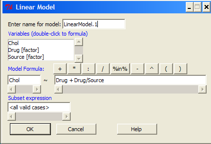
Figure 5. Nested design, linear model menu, Rcmdr, version 1.9.2
Fortunately, R and Rcmdr’s help system is quite extensive here, so when in doubt, check the help box…
Output from the linear model for the Nested Example looks like the one below.
The General Linear Model function in R and therefore Rcmdr returns information about our design plus Sums of Squares, Mean squares, and P-values. R and Rcmdr default’s to use of sequential evaluation of effects. Adjusted evaluation is useful for when you have a covariate (like body size or another confounding variable) that should be evaluated first before the factors are evaluated. We will use the sequential analysis.
Rcmdr: Models → Hypothesis tests → ANOVA table
Anova(LinearModel.15, type="II")
Anova Table (Type II tests)
Response: Chol
             Sum Sq Df F value Pr(>F)
Drug         225.14  2  1.1743 0.3262
Drug:Source  269.27  3  0.9363 0.4385
Residuals   2300.61 24
End R output
Repeatability and ANOVA
We need to tell Rcmdr how to structure the error term; you need the data frame to be arranged so
aovRes <- aov(dH2O ~ Source + Error(Source/Subject), data=SnakeTaste)
#Print the results
aovRes
Anova Table (Type II tests)
Response: dH2O
            Sum Sq Df F value   Pr(>F)
Subject     307.61  5  4.2956 0.02396 *
Source      802.78  2 28.0256 0.00007954 ***
Residuals   143.22 10
---
Signif. codes:  0 '***' 0.001 '**' 0.01 '*' 0.05 '.' 0.1 ' ' 1
#What components are available in the aovRes object?
names(aovRes)
[1] "Sum Sq"  "Df"      "F value" "Pr(>F)"
How do I extract the “F value” for Subjects?
str(aovRes)
Questions
1. What are three learning objectives from this page?
2. Be able to distinguish use of lm() and aov() and the summary output with respect to testing of linear models.
Quiz Chapter 14.8
More on the linear model in Rcmdr
Data sets
Table 1. The snake data set
| Snake | Source | flick |
| 1 | dH2O | 3 |
| 2 | dH2O | 0 |
| 3 | dH2O | 0 |
| 4 | dH2O | 5 |
| 5 | dH2O | 1 |
| 6 | dH2O | 2 |
| 1 | fish | 6 |
| 2 | fish | 22 |
| 3 | fish | 12 |
| 4 | fish | 24 |
| 5 | fish | 16 |
| 6 | fish | 16 |
| 1 | worm | 6 |
| 2 | worm | 22 |
| 3 | worm | 12 |
| 4 | worm | 24 |
| 5 | worm | 16 |
| 6 | worm | 16 |