14.1 – Crossed, balanced, fully replicated designs
Introduction
“Biology is complicated” (p. 25, National Research Council [2005]), and as researchers we need to balance our need for statistical models that fit the data well and provide insight into the phenomenon in question against compressing that complexity into ways that do not reflect the phenomenon or hinder further progress in understanding the phenomenon. From our view as researchers then, we recognize that an experiment with only one causal variable is not likely to be informative. For example, while diet has a profound effect on weight, clearly, activity levels are also important. At a minimum, when considering a weight loss program, we would want to control or monitor activity of the subjects. This is a two-factor model, the two factors diet and activity, are expected to both affect weight loss, and, perhaps, they may do so in complicated ways (e.g., on DASH diet, weight loss is accelerated when subjects exercise regularly).
Before we proceed, a word of caution is warranted. Prior to the 1990s, one could be excused for implementing experiments with simple designs that are suitable for analysis by contingency tables, t-tests, and one-way ANOVA. Now, with powerful computers available to most of us, and the feature-rich statistical packages installed on these computers, we can do much more complicated analyses on, hopefully, more realistic statistical models. This is surely progress, but caution is warranted nonetheless — just because you have powerful statistical tests available does not mean that you are free to use them — there is much to learn about the error structures of these more complicated models, for example, and how inferences are made across a model with multiple levels of interaction. In general it is preferred that experimental researchers consult and work with knowledgeable statisticians so that the most efficient and powerful experiment can be designed and subsequently analyzed with the correct statistical approach (Quinn and Keough 2002). Our introductory biostatistics textbook is not enough to provide you with all of the tools you would need and while I do advocate self-learning when it comes to statistics I do so provided we all agree that we are likely not getting the full picture this way. What we can do is provide an introduction to the field of experimental design with examples of classical designs so that the language and process of experimental design from a statistical point of view will become familiar and allow you to participate in the discussion with a statistician and read the literature as an informed consumer.
Two-factor ANOVA with replication
Our one factor statistical models can easily be extended to reflect more complicated models of causation, from one factor to two or more. We begin with two factors and the two-way ANOVA. Now we want to extend our discussion to examine how we can analyze data where we have two factors that may cause variation in the one response variable.
Consider the following two way data set.
| Diet A Population 1 |
Diet A Population 2 |
Diet B Population 1 |
Diet B Population 2 |
| 4 | 5 | 12 | 5 |
| 6 | 8 | 15 | 7 |
| 5 | 9 | 11 | 8 |
I’ve included the stacked version of this dataset at the end of this page (scroll to end or click here).
Question: What is the response variable? Which variable is the Factor variable? What are the classes of treatments and the levels of the treatments?
Answer.
Factors: Diet & Population
Levels: A, B for Diet;
Observations from population 1 or 2
Note the replication: for every level of Diet (A or B) there is an equal number of individuals from the 2 populations. Said another way, there are three replicates from population 1 for Diet A, 3 replicated from population 2 for Diet A, etc.
And finally, we say that the experiment is CROSSED: Both levels of Diet have representatives of both levels of Population.
In order to properly analyze this type of research design (2 factor ANOVA, with equal replication), the data must be crossed. “Crossed” means that each level of Factor 1 must occur in each level of Factor 2.
From the example above: each population must have individuals given diet A and diet B.
Each of the collection of observations from the same combination of Factor 1 and Factor 2 is called a CELL:
All individuals in Diet A and Population 1 are in cell 1.
All individuals in Diet A and Population 2 are in cell 2.
All individuals in Diet B and Population 1 are in cell 3.
All individuals in Diet B and Population 2 are in cell 4.
If the data is completely crossed then you can calculate the number of cells:
Number of Levels in Factor 1 x Number of Levels in Factor 2 = Total Number of Cells
From the above example: 2 Diets x 2 Populations = 4 cells.
How to analyze two factors?
One solution (but inappropriate) is to do several separate One-Way ANOVAs.
There are two reasons that this approach is not ideal:
- This approach will increase the number of tests performed and therefore will increase the chance of rejecting a Null Hypothesis when it is true (increase our p value without us being aware that it is changing – R and Rcmdr will not tell you there is a problem). This is analogous to the problems that we have seen if we perform multiple t-tests instead of a Multi-Sample ANOVA.
- More importantly, there may be interactions among the TWO Factors in how they effect the response variable. One of the more interesting possible outcomes is that the influence of one of the Factors DEPENDS on the second FACTOR. In other words, there is an interaction between factor one and factor two on how the organism responds.
Here is a graph that illustrates one possible outcome:
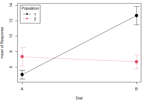
Figure 1A. One of several possible outcome of two treatments (factors). A clear interaction: First Diet level population 1 has greatest weight change, whereas for second diet level, population 2 has greatest weight change.
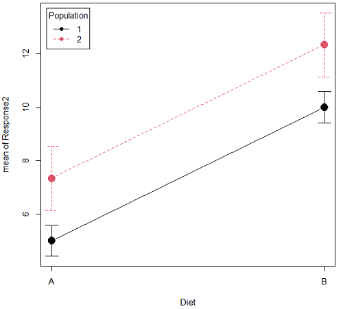
Figure 1B. One of several possible outcome of two treatments (factors). Clearly, no interaction: Population 1 always lower response than Population 2 regardless of Diet.
R code for plots
Rcmdr: Graphs → Plot of means… then added pch=19 and modified legend.pos= from "farright" to "topleft".
Figure 1A.
with(pops2, plotMeans(Response, Diet, Population, pch=19, error.bars="se", connect=TRUE, legend.pos="topleft"))
Figure 1B.
with(pops2, plotMeans(Response2, Diet, Population, pch=19, error.bars="se", connect=TRUE, legend.pos="topleft"))
Figure 1A and 1B shows that BOTH factors, Diet and Population, effect the Response of the subjects. Figure 1A also shows that the effects across Diet are not consistent: the responses are different. Individuals in Population 1 show decreased change in weight going from Diet A(1) to Diet B (2). But, individuals from Population 2 do just the opposite.
Figure 1A, because the effect of Diet cannot be interpreted without knowing which population you’re looking at, this is called an interaction between Factor 1 and Factor 2. It’s the part of the variation in the response NOT accounted for by either factor.
We can see the importance of doing the two-factor ANOVA by showing what would happen if we did two One-Factor (one-way) ANOVAs. For the first One-Factor (multi-sample) ANOVA we can examine the effect of Diet on weight. We could do this by combining the individuals from populations 1 & 2 that are given diet A (Diet A group) and then combining individuals from populations 1 & 2 that are given diet B (Diet B group).
An incorrect analysis of a two-way designed experiment
Statistical software will do exactly what you tell it to do, therefore, there is nothing to stop you from analyzing your two factor experimental design one variable at a time. It is statistical wrong to do so, but, again, there is nothing in the software that will prohibit this. So, we need to show you what happens when you ignore the experimental design in favor of a simple application of statistical analysis.
First, take a look at our two-way example with Diet as a factor and Population as another factor.
Here’s is the one-way ANOVA for Diet only.
aov(Response ~ Diet, data=pops)
| One-way ANOVA table (ignoring the other factor) |
|||||
| Source | DF | Sum of Squares | Mean Squares | F | P |
| Diet | 1 | 36.75 | 36.75 | 4.26 | 0.066 |
| Error | 10 | 86.17 | 8.62 | ||
| Total | 11 | 122.92 | |||
When we ignore (combine) the identity of the two populations in this example we see that it would APPEAR that Diet has NO EFFECT on the weight of the individuals, at least based on our statistical significance cut-off of Type I error set to 5%. Similarly, if we ignore Diet and compare responses by Population, p-value was 0.367, not statistically significant (confirm p-value from one-way ANOVA on your own).
Now let’s do the analysis correctly and pay attention to the main effect Diet.
Here’s the 2-way ANOVA table.
lm(Response ~ Diet*Population, data=pops, contrasts=list(Diet ="contr.Sum", Population
+ ="contr.Sum"))
| Two-way ANOVA (the correct analysis!) | |||||
| Source | DF | SS | MS | F | P |
| Diet | 1 | 36.75 | 36.75 | 12.25 | 0.008 |
| Population | 1 | 10.08 | 10.08 | 3.36 | 0.104 |
| Interaction | 1 | 52.08 | 52.08 | 17.36 | 0.003 |
| Error | 8 | 24.00 | 3.00 | ||
| Total | 11 | 122.92 | |||
We can visualize the results by plotting the means for each treatment group (Fig. 2).
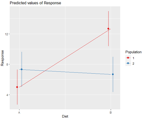
Figure 2. Plots of the main effects for Diet factor, levels A and B, and Population, levels 1 and 2.
R code for plot Fig 2A.
library(sjPlot)
library(sjmisc)
library(ggplot2)
plot_model(LinearModel.1, type = "pred", terms = c("Diet", "Population")) + geom_line()
And then for the interaction (Fig. 3).
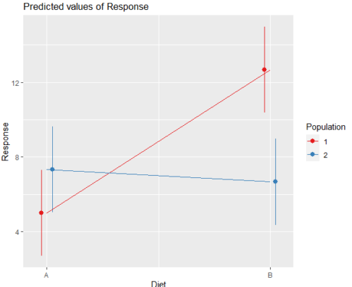
Figure 3. Interaction plot between two factors, Diet and Population.
R code: two-way ANOVA
The more general approach to running ANOVA in R is to use the general linear model function, lm(), saved as object MyLinearModel.1, for example, then follow up with
Anova(MyLinearModel.1, type="II")
to obtain the familiar ANOVA table. The lm() menu is obtained in Rcmdr by following Statistics→ Fit models→ Linear model…, and entering the model (Fig. 4). In this case, the model was

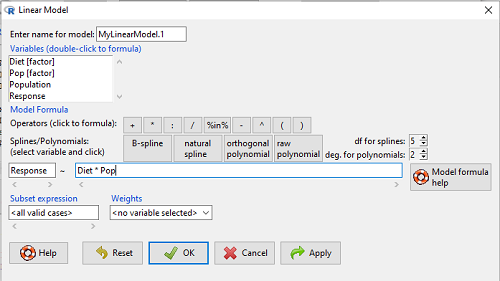
Figure 4. Linear model menu in Rcmdr.
Output from lm() function for this example

LinearModel.2 <- lm(Response ~ Diet * Pop, data=pops)
summary(LinearModel.2)

Call:
lm(formula = Response ~ Diet * Pop, data = pops)

Residuals:
Min 1Q Median 3Q Max
-2.3333 -1.1667 0.1667 1.0833 2.3333

Coefficients:
Estimate Std. Error t value Pr(>|t|)
(Intercept) 5.000 1.000 5.000 0.00105 **
Diet[T.B] 7.667 1.414 5.421 0.00063 ***
Pop[T.2] 2.333 1.414 1.650 0.13757
Diet[T.B]:Pop[T.2] -8.333 2.000 -4.167 0.00314 **
---
Signif. codes: 0 '***' 0.001 '**' 0.01 '*' 0.05 '.' 0.1 ' ' 1

Residual standard error: 1.732 on 8 degrees of freedom
Multiple R-squared: 0.8047, Adjusted R-squared: 0.7315
F-statistic: 10.99 on 3 and 8 DF, p-value: 0.003285
We want the ANOVA table, so run
Anova(MyLinearModel.1, type="II")
or in Rcmdr, Models → Hypothesis tests → ANOVA table… Accept the defaults (Types of tests = Type II, uncheck use of sandwich estimator), and press OK. I’ll leave that for you to do (see Questions).
Interaction, explained
How can we visualize the effects of the Factors and the effects of the interaction? Plot the means of a two-factor ANOVA (Fig. 5). An interaction is present if the lines cross (even if they cross outside the range of the data), but if the lines are parallel, no interaction is present.
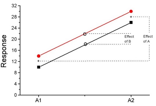
Figure 5. A plot showing no interaction between factor A and factor B for some ratio scale response variable.
A large effect of factor A – compare means
A small effect of factor B – compare means
Little or no interaction – lines are parallel
Three hypotheses for the Two-Factor ANOVA
The important advance in our statistical sophistication (from one to two factors!!) allows us to ask three questions instead of just two question:
- Is there an effect of Factor 1?
- HO: There is no effect of Factor 1 on the response variable.
- HA: There is an effect of Factor 1 on the response variable.
- Is there an effect of Factor 2?
- HO: There is no effect of Factor 2 on the response variable.
- HA: There is an effect of Factor 2 on the response variable.
- Is there an INTERACTION between Factor 1 & Factor 2?
- HO: There is no interaction between Factor 1 & Factor 2 on the response variable.
- HA: There is an interaction between Factor 1 & Factor 2 on the response variable.
Questions
- In the crossed, balanced two-way ANOVA, how many Treatment groups are there if Factor 1 has three levels and Factor 2 has four levels?
A. 3
B. 4
C. 7
D. 9
E. 12 - What is meant by the term “balanced” in a two-way ANOVA design?
A. Within levels of a factor, each level has the same sample size
B. Each level of one factor occurs in each level of the other factor
C. There are no missing levels of a factor.
D. Each level of a factor must have more than one sampling unit. - What is meant by the term “crossed” in a two-way ANOVA design?
A. Within levels of a factor, each level has the same sample size
B. Each level of one factor occurs in each level of the other factor
C. There are no missing levels of a factor.
D. Each level of a factor must have more than one sampling unit. - What is meant by the term “replicated” in a two-way ANOVA design?
A. Within levels of a factor, each level has the same sample size
B. Each level of one factor occurs in each level of the other factor
C. There are no missing levels of a factor.
D. Each level of a factor must have more than one sampling unit. - Use the multi-way ANOVA command in
Rcmdrto generate the ANOVA table for the example data set. - Use the linear model function and Hypothesis tests in
Rcmdrto generate the ANOVA table for the example data set.
Quiz Chapter 14.1
Crossed, balanced, fully replicated designs
Data set
Don’t forget to convert the numeric Population variable to character factor, e.g., a new object called Pop. The R command is simply
Pop <- as.factor(Population)
But easy to use Rcmdr also. From within Rcmdr select Data → Manage variables in active dataset → Convert numeric variables to factors…
| Diet | Population | Response |
| A | 1 | 4 |
| A | 1 | 6 |
| A | 1 | 5 |
| A | 2 | 5 |
| A | 2 | 8 |
| A | 2 | 9 |
| B | 1 | 12 |
| B | 1 | 15 |
| B | 1 | 11 |
| B | 2 | 5 |
| B | 2 | 7 |
| B | 2 | 8 |