7.2 – Epidemiology basics

Introduction
Prevalence rate
Prevalence: R code
Incidence rate
Person-time
Incidence rate: R code
Age-specific rates
Age-adjusted rates
Questions
Chapter 7 contents

Introduction

To introduce conditional probability, I have elected to push you into epidemiology and risk analysis. We introduced epidemiology definitions and here, we build on basic terminology of epidemiology. Epidemiology is the study of the causes and distribution of health-related events in a population. It is has been called the basic science of public health (p. 16, Decker 2008).

Prevalence rate

Prevalence of a disease (or condition), is defined as the proportion of the population that has the disease (condition) at a point or duration in time. The prevalence statistic is the ratio of the number of existing cases divided by the total population.

For example, let’s say we’re interested in the prevalence of Type 2 diabetes in Hawai`i. The 2020 populations was about 1.4 million. A survey is conducted on a random of 1000 individuals and 80 were reported to have Type 2 diabetes. What is the estimated prevalence of Type 2 diabetes in Hawai`i?

Start from perspective — what if we actually have something close to a census count? For the actual estimates, see the report at the Hawaii State DOH website. With every estimate of a statistic, we need a confidence interval (CI). An approximate (good for large samples) formula for the 95% CI of prevalence is

$\begin{align*} 95\% \ CI=\hat{p}\pm z \sqrt{\frac{1}{N}\hat{p}\left (1-\hat{p} \right )} \end{align*}$

where $\hat{p}$ is the 2010 prevalence in the population (8.3%), N is the population size (1,360,301), and z is the standard normal probability. For a 95% CI, then we want z_95%.

If you recall, we can get this from our standard normal probability table, or directly from R. We want to know z that is in the ± 2.5% tails of the distribution (that’s 0.05 ÷ 2, see Ch 8.4 – Tails of a test). Our R code then is

qnorm(c(0.025), mean=0, sd=1, lower.tail=FALSE)

which returns

[1] 1.959964

You should confirm that setting lower-tail = TRUE yields -1.96 (rounded).

Alternately, if using Rcmdr: Distributions → Continuous distributions → Normal distribution → Normal quantiles… (Fig. 1)

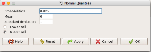
Figure 1. R Commander popup menu for Normal quantiles.

Figure 1. R Commander popup menu for Normal quantiles.

Thus, for our example, the 95% CI was ( $8.3 - 0.046, 8.3, + 0.046)$ ; our confidence in our estimate of the prevalence of diabetes in Hawaii is between 8.25% and 8.35%. Again, note that for our purposes it is OK to calculate the approximate confidence interval, replace $\pm 1.96$ with $2$ (for large N, the differences are observed in the 0.001 decimal).

Prevalence: R code

Rather than census counts, more likely we have results of smaller surveys. We use the epi.conf() function from the epiR package. Code adapted from example provided in epiR_descriptive vignette.

Note. Many R packages include vignettes, which, together with the package manual, is often helpful to understand what a function is intended to do and how to get the most from the function. R code to call all vignettes available for a package, e.g., epiR:

vignette(package="epiR")

which will return names of available vignettes. For epiR, these are

epiR_descriptive Descriptive epidemiology (source, html)
epiR_surveillance Disease surveillance (source, html)
epiR_measures_of_association Measures of association (source, html)
epiR_sample_size Sample size calculations (source, html)

To call up the vignette we need for this example,

vignette("epiR_descriptive", package="epiR")

which brings up the page (assuming you installed the html help files during installation of base R).

library(epiR)
pop.Hawaii = 1.4e06
pop.Survey = 1000
type2.Survey = 80 
Table.2 <- as.matrix(cbind(type2.Survey, pop.Survey)) 
epi.conf(Table.2, ctype = "prevalence", method = "exact", N = pop.Hawaii, design = 1, conf.level = 0.95) * 100

R output

   est    lower    upper
1    8 6.394198 9.857978

Thus, estimated Type 2 diabetes prevalence from the survey was 8, with 95% confidence interval 6.4 to 9.9 cases per 100 individuals. From 2020 U.S. Census, Hawai`i population was 1,455,271.

Note. Type 2 diabetes is one of many conditions for which prevalence is greater among Native Hawaiian and Pacific Islander populations compared to other groups in Hawai’i (Galinski et al 2016); these are called health disparitiess.

Incidence rate

Incidence of a disease (or condition) is defined as the occurrence of new cases of a disease. The simplest way to view incidence is that if everyone was followed for the same period of time, then incidence rate is the number of new cases since the start of the study divided by the total population. This is too simplistic, so we define a better metric called person-time. Incidence rate (IR) is then the ratio of the number of new cases divided by total person-time.

Again, incidence rate is an estimate. Therefore, we need a confidence interval. Assuming the population is large, then confidence interval can be calculated as

$\begin{align*} IR\pm z\sqrt{\frac{N}{T^{2}}} \end{align*}$

where IR is the incidence rate, T is the person-time, N is the number of events or cases, and z again is the standard normal probability (z ± 1.96 for 95% confidence interval).

For our example, N = 3 cases, T = 236 p-d, so 95% CI is (11.3%, 14.1%).

Person-time

Person-time can be days, months, years. Person-time is best defined with an example.

Five men join a study that will last 70 days. These men were selected because they had suffered a myocardial infarction (MI) and at the start of the study, they receive the same treatment. The outcome of the study is whether or not the subjects suffer a second MI.

The results are shown below

Subject A, 53 days
Subject B, 70 days
Subject C, 24 days
Subject D, 70 days
Subject E, 19 days

Add up the person days,

$\begin{align*} 53+70+24+70+19=236 \ person-days\left (p-d \right ) \end{align*}$

Now calculate the incidence rate,

$\begin{align*} 1000\cdot \frac{3 \ cases}{236p-d}=12.7 \ person-days \end{align*}$

that’s 3 cases (A, C, E) divided by 236 p-d = 0.0127. Multiply this by 1000 and we get our final answer for the incidence rate, 12.7 per person-days.

Incidence rate: R code

Incidence rate of myocardial infarction (MI) study. Code adapted from example provided in epiR_descriptive vignette.

ncas = 3
ntar = 236
tmp <- as.matrix(cbind(ncas, ntar))
epi.conf(tmp, ctype = "inc.rate", method = "exact", N = 1000, design = 1, conf.level = 0.95) * 1000

R output

          est    lower    upper
ncas 12.71186 2.621492 37.14946

The incidence rate of myocardial infarction was 12.7 (95% CI 2.6 to 37.2) cases per 1000 person-days.

Age-specific rates

Incidence or prevalence rates may be reported for specific age groups. For example, we can distinguish between number of live births in Hawaii in 2017, and numbers of live births by age group of the mother.

Age-adjusted rates

If populations with different age demographics, then the convention is to adjust the populations to a standard reference population with known age and other demographic properties. For example, the CDC uses the 2000 census as the standard population (CDC definitions, age adjustment, retrieved January 2023).

Questions

Calculate the confidence interval of type 2 prevalence in Hawai`i with the 2020 census population value. How much did it change?
Recalculate the confidence interval for a 99% confidence interval. Which estimate communicates greater confidence in the estimate?