20.6 – Dimensional analysis
draft
Introduction
Cluster analysis or clustering is a multivariate analysis technique that includes a number of different algorithms for grouping objects in such a way that objects in the same group (called a cluster) are more similar to each other than they are to objects in other groups. A number of approaches have been taken, but loosely can be grouped into distance clustering methods (see Chapter 16.6 – Similarity and Distance) and linkage clustering methods: Distance methods involve calculating the distance (or similarity) between two points and whereas linkage methods involve calculating distances among the clusters. Single linkage involves calculating the distance among all pairwise comparisons between two clusters, then
Cluster analysis is common to molecular biology and phylogeny construction and more generally is an approach in use for exploratory data mining. Unsupervised machine learning (see 20.14 – Binary classification) used to classify, for example, methylation status of normal and diseased tissues from arrays (Clifford et al 2011)
Results from cluster analyses are often displayed as dendograms. Clustering methods include a number of different algorithms hierarchical clustering: single-linkage clustering; complete linkage clustering; average linkage clustering (UPGMA) centroid based clustering: k-means clustering
R packages
factoextra
MorphoFun/psa/
Principal component analysis
Bumpus data from MorphoFun/psa, variable names changed.
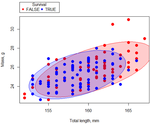
Figure ccc. Scatterplot English swallow mass (g) by total length (mm) by survival following winter storm
R code for graph
scatterplot(Weight~Total_length | Survival, regLine=FALSE, smooth=FALSE, boxplots=FALSE,
ellipse=list(levels=c(.9)), by.groups=TRUE, grid=FALSE, pch=c(19,19), cex=1.5, col=c(“red”,”blue”), xlab=”Total length, mm”, ylab=”Mass, g”, data=Bumpus)
Data ellipse — 90% of the pairwise points (red, did not survive; blue, did survive), not a confidence ellipse
Bumpus measured several traits, we want to use all of the data. However, highly correlated.
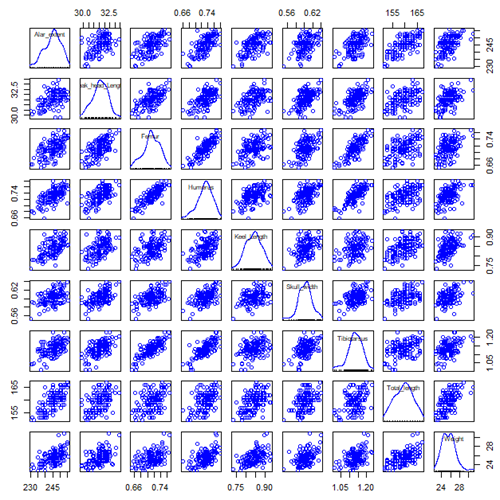
Figure ccc. Scatterplot matrix of Bumpus English sparrow traits. Traits were (left-right): Alar extent (mm), length (tip of beak to tip of tail), length of head (mm), length of femur (in.), length of humerus (in.), length of sternum (in.), skull width (in.), length of tibio-taurus (in.), and weight (g)
R code for graph
scatterplotMatrix(~Alar_extent+Beak_head_Length+Femur+Humerus+Keel_Length+Skull_width+Tibiotarsus+Total_length+Weight, regLine=FALSE, smooth=FALSE, diagonal=list(method=”density”), data=Bumpus)
Note. In Chapter 4, we discussed importance of white space and Y-scale for graphs that make comparisons. Figure ccc is a good example of where we trade-off the need for white space and concerns about telling the story — the various traits are positively correlated — against the dictum of an equal Y-scale for true comparisons.
Rcmdr: Statistics > Dimensional analysis > Principal component analysis …
.PC <-
princomp(~Alar_extent+Beak_head_Length+Femur+Humerus+Keel_Length+Skull_width+Tibiotarsus+Total_length+Weight, cor=TRUE, data=Bumpus)
cat(“\nComponent loadings:\n”)
print(unclass(loadings(.PC)))
cat(“\nComponent variances:\n”)
print(.PC$sd^2)
cat(“\n”)
print(summary(.PC))
screeplot(.PC)
Bumpus <<- within(Bumpus, {
PC2 <- .PC$scores[,2]
PC1 <- .PC$scores[,1]
})
})
Importance of components
Comp.1 Comp.2
Standard deviation 2.3046882 0.9988978
Proportion of Variance 0.5901764 0.1108663
Cumulative Proportion 0.5901764 0.7010427
K-means clustering
Number of clusters
Iterations
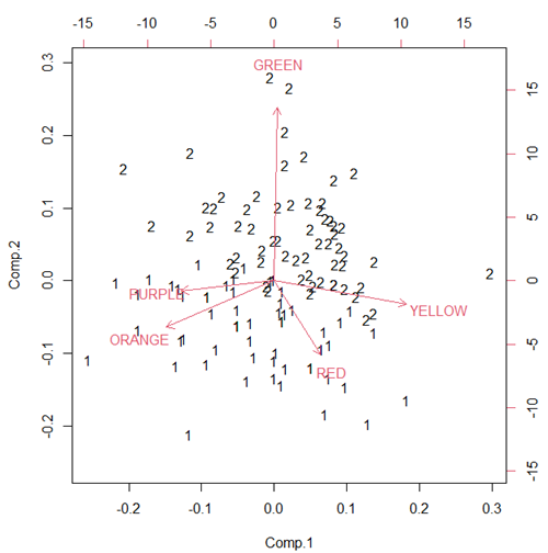
Figure ccc. Bi-plot of clusters, Skittles mini bags
Hierarchical clustering
Ward’s method
Complete linkage
McQuitty’s method
Centroid linkage
A common way to depict the results of a cluster analysis is to construct a dendogram.
Questions
[pending]
References and further reading
Clifford, H., Wessely, F., Pendurthi, S., & Emes, R. D. (2011). Comparison of clustering methods for investigation of genome-wide methylation array data. Frontiers in genetics, 2, 88.
Ferreira, L., & Hitchcock, D. B. (2009). A comparison of hierarchical methods for clustering functional data. Communications in Statistics-Simulation and Computation, 38(9), 1925-1949.
Fraley C, Raftery AE. (2002) Model-based clustering, discriminant analysis, and density estimation. J Am Stat Assoc. 2002; 97(458):611–31.
Chapter 20 contents
- Additional topics
- Area under the curve
- Peak detection
- Baseline correction
- Surveys
- Time series
- Cluster analysis
- Estimating population size
- Diversity indexes
- Survival analysis
- Growth equations and dose response calculations
- Plot a Newick tree
- Phylogenetically independent contrasts
- How to get the distances from a distance tree
- Binary classification
/MD