10.1 – Compare two independent sample means
Introduction
We introduced the concept of comparing a sample statistic (mean) against a population parameter (Chapter 6.7, Normal deviate) or one-sample t-test against a specified mean (eg, from published data or from theory, Chapter 8.5).
Consider now a basic experimental design, the randomized control trial, or RCT (Fig 1), introduced in Chapter 2.4.
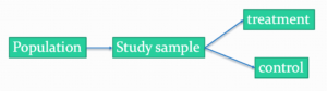
Figure 1. A two group Randomized Control Trial.
Subjects randomly selected from population of interest, then again — random assignment — once recruited into one of two treatment groups. Importantly, subjects belong to one treatment arm only: no subject simultaneously receives the treatment and the control. This is in contrast to the paired design, in which subjects receive both treatments (see Chapter 10.3).
In inferential statistics about an experiment, we are more likely trying to test if sample means are different. For example
- two species grown in common garden, do they differ in growth rate?
- human subjects given a new treatment have better outcomes compare to those receiving a control treatment (eg, placebo).
The equivalent null hypothesis is that two samples are pulled from the same population. We write the null hypothesis as

and the corresponding alternative hypothesis, HA, then must be

Question: Is this a one tailed or two-tailed hypothesis?
Answer: Two-tailed (review Chapter 8.4)
Note 1: In this day and age, there’s really no compelling reason to learn the t-test. First, it is just a special case of the one-way ANOVA, therefore, it’s a special case of the general linear model. Struggling to learn R commands? Well, one solution would be just to learn the general linear model approach — the R function lm() (OK — don’t get too excited — lm() has many options and details). Second, few experiments or observational studies are likely to have only two groups; thus, the temptation to carry out a series of t-tests, taking all groups two at a time, or “pairwise,” while tempting, actually violates a whole bunch of basic statistical rules (discussed in Chapter 12.1). It will also make statisticians go crazy when they see it. That said, if your experiment has but two groups, then by all means, the t-test is a choice. The t-test is also a statistical test that you have likely already used before so we present the discussion here to build on what you may already have learned. We also present the independent t-test as a vehicle.
Worked example
We introduce the two-sample t-test, or better, the independent sample t-test.

where the numerator is the difference between the two sample means and the denominator is the standard error of the differences between the two groups standard errors. The formula for

The choice of independent sample over two-sample is best because it emphasizes that the two groups (the two samples), must be comprise of independent sampling units. This is a pretty straight-forward requirement; you have randomly assigned twenty individuals to two groups, a control group (n = 10) and a treatment group (n = 10). Individuals are either in the control group or they are in the treatment group — they cannot simultaneously appear in both groups.
We will work our way through this test by example. For starters, let’s use the same lizard dataset (see Example data set, below), four body mass recordings (grams) each for house geckos (Hemidactylus frenatus, Fig 2) and the Carolina anole (Anolis carolensis, Fig 3), two of many lizard species introduced to Hawaiʻi.

Figure 2. Male Hemidactylus frenatus, central Oahu, M. Dohm.

Figure 3. Male Anolis carolinensis, ʻAkaka Falls, Big Island of Hawaiʻi, M. Dohm.
Example data set
Geckos: 3.186, 2.427, 4.031, 1.995

Anoles: 5.515, 5.659, 6.739, 3.184
Question: How would you go about creating a data frame with the values in long form (stacked worksheet), including a label variable and the body mass?
Note 2: The independent sample t-test in Rcmdr requires a stacked worksheet and not in unstacked worksheet two columns implied by the above pseudo-code. If you need help with worksheet format, then see Part07 in Mike’s Workbook for Biostatistics.
Answer: At the R prompt, type
Geckos <- c(3.186, 2.427, 4.031, 1.995); Anoles = c(5.515, 5.659, 6.739, 3.184) #create two vectors
bmass <- c(Geckos, Anoles)    #combine the two vectors into a single vector holding all of the body mass records
species <- c("gecko", "gecko", "gecko", "gecko", "anole", "anole", "anole", "anole")   #create your label variable
lizards <- data.frame(species, bmass)  #create your data frame
lizards   #print your data frame  species bmass
1   gecko 3.186
2   gecko 2.427
3   gecko 4.031
4   gecko 1.995
5   anole 5.515
6   anole 5.659
7   anole 6.739
8   anole 3.184
Note also that you can enter data into the Data editor by creating the data frame first then adding values. To edit the data frame “lizards” type fix(lizards) at the R prompt, then close the data frame when you have added or changed values as needed.
As always, begin with an exploration of the data, including a graph (Fig 4).
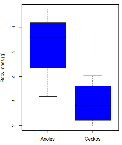
Figure 4. Box plot of lizard body mass.
We can see already that there’s greater spread of data for the Anoles compared to the Geckos, but the median values differ. Small sample sizes can be a problem for analyses as we can only have reduced confidence in our conclusions. However, we press on for the sake of demonstration.
Let’s test the null hypothesis, H0, i.e., the two species of lizards have the same mean body mass.
Rcmdr: Statistics → Means → Independent-samples t-test…
In this next image I posted the Rcmdr menu popup for the Independent Samples t-test (Fig 5). Later versions of Rcmdr split the settings for this command into two tabs; the first tab allows for the selection of the variables and setting the hypotheses whereas the second tab, labeled Options, permits additional choices. The default selections need your attention: to actually conduct the t-test you need to answer “No” to the question, “Assume equal variance?” (Fig 6).
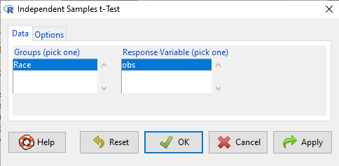
Figure 5. Rcmdr menu for Independent sample t-test.
Select the Options tab (Fig 6) to select null hypothesis and to select the t-test and not the Welch-test (which is the default, i.e., No to the prompt “Assume equal variances?”).
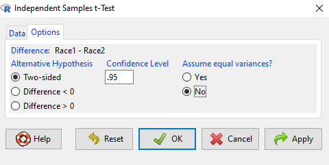
Figure 6. Rcmdr Options menu for Independent sample t-test.
Let’s look at the results and break down the parts of the test.
t.test(Body.mass~Lizard, alternative='two.sided', conf.level=.95,
+ var.equal=TRUE, data=lizards)

Two Sample t-test

data: Body.mass by Lizard
t = 2.7117, df = 6, p-value = 0.03503
alternative hypothesis: true difference in means is not equal to 0
95 percent confidence interval:
0.2308685 4.4981315
sample estimates:
mean in group Anolis mean in group Gecko
5.27425 2.90975
Consider the R session output above and answer the following questions.
Questions for the worked example
- Which lizard group had the greater mean value, Anolis or Gecko?
- What are the assumptions necessary for you to use the independent sample t-test?
- What does “two-sided” mean?
- What was the null hypothesis?
- Was this a one-tailed or two-tailed test of the null hypothesis?
- What is the value of the test statistic?
- How many degrees of freedom?
- What is the critical value for this test?
- What is the value of the lower limit of the 95% confidence interval?
- What is the value of the lower limit of the 99% confidence interval?
- True or False. If the null hypothesis is accepted, then zero is a value included in the 95% confidence interval.
- Do you accept the null hypothesis? Explain your selection.
Try another example
DNA damage, changes in the chemical structure of nucleotide bases or breakage of the DNA chains, occurs in cells under many circumstances. The comet assay, or single-cell gel electrophoresis, is one method for visualizing and measuring DNA strand breaks in cells. Exposed cells are mixed with a low-melting temperature agarose and placed onto a microscope slide. The cells are then lysed with an alkaline detergent and high salts. When current is applied across the slide, undamaged DNA remains in the nucleus, whereas damaged DNA extends towards the anode to form a comet-like tail, with imaging assisted by including a fluorescent dye like Sybr-Green. Examples of comets are shown below (Fig 7).
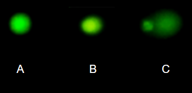
Figure 7. Comet examples. A Intact cell, no DNA damage, B Cell with some DNA damage, a slight tail to the right is evident, C Cell with significant DNA damage, a large tail is evident. M. Dohm.
In an experiment, immortalized lung epithelial cells were exposed to dilute copper solutions for 30 minutes then washed with PBS. The comet assay was applied to these cells and for comparison, to cells without copper exposure but otherwise treated the same way (controls). The data are available at the bottom of this page (scroll down or click here).
Again, you should begin all analyses with an exploration of the data, including a graph (Fig 8).
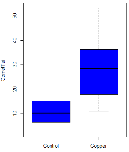
Figure 8. Boxplot of comet tail lengths for cells with and without (control) exposure to copper in the cell medium for 30 minutes.
Let’s look at the R output for the t-test analysis.
    Two Sample t-test

data:  CometTail by Treatment
t = -5.8502, df = 38, p-value = 9.139e-07
alternative hypothesis: true difference in means is not equal to 0
95 percent confidence interval:
 -22.39865 -10.88213
sample estimates:
mean in group Control  mean in group Copper
             11.14533              27.78571
Consider the R session output above and answer the following questions.
Questions for Comet assay data set
- Which cell group had the greater mean value, Copper-exposed or Control-exposed cells?
- What are the assumptions necessary for you to use the independent sample t-test?
- What does “two-sided” mean?
- What was the null hypothesis?
- Was this a one-tailed or two-tailed test of the null hypothesis?
- What is the value of the test statistic?
- How many degrees of freedom?
- What is the critical value for this test?
- What is the value of the lower limit of the 95% confidence interval?
- What is the value of the lower limit of the 99% confidence interval?
- True or False. If the null hypothesis is accepted, then zero is a value included in the 95% confidence interval.
- Do you accept the null hypothesis? Explain your selection.
T test from summary statistics
In some cases you may only have to summary statistics for data, eg, the means and the standard deviations. We can use the equations of the t test to write a simple formula, where the user provides the known means, standard deviations, and sample size. For example, create a simple function with readline for user input.
myTtest <- function() {
   mnx <- as.numeric(readline(prompt="Enter mean of x: "))
   stdevx <- as.numeric(readline(prompt="Enter sd of x: "))
   nx <- as.numeric(readline(prompt="Enter n of x: "))
   mny <- as.numeric(readline(prompt="Enter mean of y: "))
   stdevy <- as.numeric(readline("Enter sd of y: "))
   ny <- as.numeric(readline(prompt="Enter n of y: "))
   myTvalue <- abs(((mnx-mny)-0)/sqrt(((stdevx^2)/nx)+(stdevy^2)/ny))
   myDF <- as.integer(nx+ny-2)
   myPvalue <- pt(myTvalue,myDF,lower.tail=FALSE)*2
   myResults <- c(myTvalue, myDF, myPvalue)
   report <- c("T-test: ", "df: ", "two-tailed p-value: ")
   cat(sprintf("%s %3.3f, ", report, myResults))
}
then run the function by typing myTest() at the R prompt and entering the means, standard deviations, and sample size when prompted.
myTtest()
Enter mean of x: 2.91
Enter sd of x: .895
Enter n of x: 4
Enter mean of y: 5.27
Enter sd of y: 1.497
Enter n of y: 4
T-test: 2.706, df: 6.000, two-tailed p-value: 0.035
P-values from confidence intervals
While we expect certain reporting criteria for published, it is not uncommon that one or more elements are missing. For example, while means plus or minus standard deviations for two groups may be reported, the confidence interval of the difference may not be reported, or, an inexact p-value is reported like “< 0.05,” but we “need” an exact p-value for our meta-analysis. A little math, and these missing statistics can be calculated.
We can use the lizard study as an example; while all of the expected elements were reported, including the p-value (0.03503), let’s say the p value was reported as “statistically significant at p < 0.05.”
We need
lower and upper confidence intervals: 0.2309 and 4.498, respectively.
critical value from t distribution, df = 6 (2 tailed, therefore 0.05/2). A little R code we have:

the standard error, which can be calculated as 
and then the p-value, 
which is pretty close to the result from R (p = 0.03503). The difference is likely due to the small sample size.
Questions
- Don’t forget to work through the Questions for the Comet tail data set (scroll up or click here).
- Microsoft Excel, LibreOffice Calc, and Google sheets spreadsheet software all include t-test functions and return the p-value. Consider two variables big (100, 110, 120, 100, 110, 210, 200) and small (0,1,1,2,0,1,0). (Note — these two groups are obviously very different, calculating a t-test on their difference is silly, just for this question.) If formatting is set to the default two decimal places for Number cell category, the p-value will return as “0.00.” How should you report the p-value in this case?
Quiz Chapter 10.1
Compare two independent sample means
Comet assay data set
| Treatment | CometTail |
| Control | 17.856139 |
| Control | 16.52125 |
| Control | 14.925449 |
| Control | 14.029174 |
| Control | 13.332945 |
| Control | 8.811185 |
| Control | 14.701654 |
| Control | 9.261025 |
| Control | 21.779311 |
| Control | 6.180284 |
| Control | 9.201752 |
| Control | 5.54472 |
| Control | 6.717885 |
| Control | 2.625092 |
| Control | 7.191583 |
| Control | 5.392866 |
| Control | 11.284813 |
| Control | 15.441254 |
| Control | 17.857176 |
| Control | 4.250956 |
| Copper | 53.214287 |
| Copper | 38.92857 |
| Copper | 18.928572 |
| Copper | 30 |
| Copper | 28.928572 |
| Copper | 15.357142 |
| Copper | 17.857143 |
| Copper | 17.5 |
| Copper | 21.071428 |
| Copper | 29.285715 |
| Copper | 28.214285 |
| Copper | 16.785715 |
| Copper | 21.071428 |
| Copper | 37.5 |
| Copper | 38.214287 |
| Copper | 17.857143 |
| Copper | 29.642857 |
| Copper | 11.071428 |
| Copper | 35 |
| Copper | 49.285713 |
Chapter 10 contents
- Introduction
- Compare two independent sample means
- Digging deeper into t-test Plus the Welch test
- Paired t-test
- References and suggested reading