17.5 – Testing regression coefficients

Introduction
Linear regression inference
R code
Test two slopes
Example
Questions
Chapter 17 contents

Introduction

Whether the goal is to create a predictive model or an explanatory model, then there are two related questions the analyst asks about the linear regression model fitted to the data:

Does a line actually fit the data
Is the linear regression statistically significant?

We will turn to the first question pertaining to fit in time, but for now, focus on the second question.

Like the one-way ANOVA, we have the null and alternate hypothesis for the regression model itself. We write our hypotheses for the regression

H₀ : linear regression fits the data vs. H_A : linear regression does not fit

We see from the output in R and Rcmdr that an ANOVA table has been provided. Thus, the test of the regression is analogous to an ANOVA — we partition the overall variability in the response variable into two parts: the first part is the part of the variation that can be explained by there being a linear regression (the linear regression sum of squares) plus a second part that accounts for the rest of the variation in the data that is not explained by the regression (the residual or error sum of squares). Thus, we have

$\begin{align*} SS_{Total} = SS_{regression} + SS_{residual} \end{align*}$

As we did in ANOVA, we calculate Mean Squares $MS_{x}= SS_{x}/DF_{x}$ , where x refers to either “regression” or “residual” sums of squares and degrees of freedom. We then calculate F-values, the test statistics for the regression, to test the null hypothesis.

The degrees of freedom (DF) in simple linear regression are always

$\begin{align*} DF_{total} = n - 1 DF_{regression} = 1 DF_{residual} = DF_{total} - DF_{regression} = n - 2 \end{align*}$

where

$\begin{align*} F = \frac{MS_{regression}}{MS_{residual}} \end{align*}$

and F_DFregression, DF_residual are compared to the critical value at Type I error rate α, with DFregression, DFresidual.

Linear regression inference

Estimation of the slope and intercept is a first step and should be accompanied by the calculation of confidence intervals.

What we need to know if we are to conclude that there’s a functional relationship between the X and Y variable is whether the same relationship exists in the population. We’ve sampled from the population, calculated an equation to describe the relationship between them. However, just as in all cases of inferential statistics, we need to consider the possibility that, through chance alone, we may have committed a Type I error.

The graph below (Fig. 1) shows a possible outcome under a scenario in which the statistical analyst would likely conclude that there is a statistically significant linear model fit to the data, but the true relationship in the population was a slope of zero. How can this happen? Under this scenario, by chance alone the researchers sampled points (circled in red) from the population that fall along a line. We will conclude that there is linear relationship — that’s what are inferential statistics work would indicate — but there was none in the population from which the sampling was done; there would be no way for us to recognize the error except to repeat the experiment — the principal of research reproducibility — with a different sample.

Scatterplot of hypothetical x,y data for which the researcher may obtain a statistically significant linear fit to sample of data from population in which null hypothesis is true relationship between x and y.

Figure 1. Scatterplot of hypothetical x,y data for which the researcher may obtain a statistically significant linear fit to sample of data from population in which null hypothesis is true relationship between x and y.

So in conclusion, you must keep in mind the meaning of statistical significance in the context of statistical inference: it is inference done on a background of random chance, the chance that sampling from the population leads to a biased sample of subjects.

Note: If you think about what I did with this data for Figure 1 graph, purposely selecting data that showed a linear relationship between Y and X (red circles), then you should recognize this as an example of data dredging or p-hacking, cf. discussion in Head et al (2015); Stefan and Schönbrodt (2023). However, the graph is supposed to be read as if we could do a census and therefore have full knowledge of the true relationship between y and x. The red circles indicate the chance that sampling from a population may sometimes yield incorrect conclusions.

Tests of coefficients

One criterion for a good model is that the coefficients in the model, the intercept and the slope(s) are all statistically significant.

For the statistical of the slope, b₁, we generally treat the test as a two-tailed test of the null hypothesis that the regression slope is equal to zero.

H₀ : b₁ = 0 vs. H_A : b₁ ≠ 0

Similarly, for the statistical of the intercept, b₀, we generally treat the test as a two-tailed test of the null hypothesis that the Y-intercept is equal to zero.

H₀ : b₀ = 0 vs. H_A : b₀ ≠ 0

For both slope and intercept we use t-statistics.

$\begin{align*} t = \frac{b}{SE_{b}} \end{align*}$

We’ll illustrate the tests of the slope and intercept by letting R and Rcmdr do the work. You’ll find this simple data set at the bottom of this page (scroll or click here). The first variable is the number of matings, the second is the size of the paired female, and the third is the size of the paired male. All body mass were in grams.

R code

After loading the worksheet into R and Rcmdr, begin by selecting

Rcmdr: Statistics → Fit model → Linear Regression

Note that more than one predictor can be entered, but only one response (dependent) variable may be selected (Fig. 2).

Screenshot Rcmdr linear regression menu. Select one response variable and one or more explanatory variables

Figure 2. Screenshot linear regression menu. More than explanatory (predictor or independent) variables may be selected, but only one response (dependent) variable may be selected.

This procedure will handle simple and multiple regression problems. But before we go further, answer these two questions for the data set.

Question 1. What is the Response variable?

Question 2. What is the Explanatory variable?

Answers. See below in the R output to see if you were correct!

If there is only one predictor, then this is a Simple Linear Regression; if more than one predictor is entered, then this is a Multiple Linear Regression. We’ll get some more detail, but for now, identify and evaluate the test (p-value) of the slope coefficient (labeled after the name of the predictor variable), the test of the intercept coefficient, and some new stuff.

R output

RegModel.1 <- lm(Matings ~ Female, data=birds)
summary(RegModel.1)
Call: lm(formula = Matings ~ Female, data = birds) 
Residuals: 
     Min       1Q     Median         3Q        Max 
-2.32805 -1.59407   -0.04359    1.77292    2.67195 

Coefficients: 
              Estimate    Std. Error     t value    Pr(>|t|) 
(Intercept)    -8.6175        3.5323      -2.440     0.02528 * 
Female          0.3670        0.1042       3.524     0.00243 ** 
--- 
Signif. codes: 0 '***' 0.001 '**' 0.01 '*' 0.05 '.' 0.1 ' ' 1 
Residual standard error: 1.774 on 18 degrees of freedom 
Multiple R-squared: 0.4082, Adjusted R-squared: 0.3753 F-statistic: 12.42 on 1 and 18 DF, p-value: 0.002427

In this example, slope = 0.367 and the intercept = -8.618. The first new term we encounter is called Multiple R-squared (R²) — it’s also called the coefficient of determination. It’s the ratio of the sum of squares due to the regression to the total sums of squares. R² ranges from zero to 1, with a value of 1 indicating a perfect fit of the regression to the data.

If you are looking for a link between correlation and simple linear regression, then here it is: R² is the square of the product-moment correlation, r. Thus, r = √R² see Chapter 17.2).

We introduced $R^2$ in Chapter 17.1 . Interpretation of R² goes like this: If R² is close to zero, then the regression model does not explain much of the variation in the dependent variable; conversely, if R² is close to one, then the regression model explains a lot of the variation in the dependent variable.

Did you get the Answers?

Answer 1: Number of matings

Answer 2: Size of females

Interpreting the output

Recall that

$\begin{align*} SS_{Total} = SS_{regression} + SS_{residual} \end{align*}$

then

$\begin{align*} R_{2}= {SS_{regression}}{SS_{Total}} \end{align*}$

From the output we see that R² was 0.408, which means that about 40% of the variation in numbers of matings may be explained by size of the females alone.

To complete the analysis get the ANOVA table for the regression.

Rcmdr: Models → Hypothesis tests → ANOVA table…

> Anova(RegModel.1, type="II") 
Anova Table (Type II tests) 
            Sum Sq   Df   F value      Pr(>F) 
Female      39.084    1    12.415    0.002427 ** 
Residuals   56.666   18 
--- 
Signif. codes: 0 '***' 0.001 '**' 0.01 '*' 0.05 '.' 0.1 ' ' 1

With only one predictor (explanatory) variable, note that the regression test in the ANOVA is the same (has the same probability vs. the null hypothesis) as the test of the slope.

Test two slopes

A more general test of the null hypothesis involving the slope might be

H₀ : b₁ = b vs. H_A : b₁ ≠ b

where b can be any value, including zero. Again, t-test would then be used to conduct the test of the slope, where the t-test would have the form

$\begin{align*} t = \frac{b_{1} - b_{2}}{SE_{b_{1} - b_{2}}} \end{align*}$

where SE_b1-b2 is the standard error of the difference between the two regression coefficients. We saw something similar to this value back when we did a paired t-test. To obtain s_b1–_b2, we need the pooled residual mean square and the squared sums of the X values for each of our sample.

First, the pooled (hence the subscript p) residual mean square is calculated as

$\begin{align*} \left (s_{y \cdot x}^2 \right )_{p} = \frac{resSS_{1}}{resDF_{1}} + \frac{resSS_{2}}{resDF_{2}} \end{align*}$

where resSS and resDF refer to residual sums of squares and residual degrees of freedom for the first (1) and second (2) regression equations.

Second, the standard error of the difference between regression coefficients (squared!!) is calculated as

$\begin{align*} s_{b1-b2} = \left (s_{y \cdot x}^2 \right )_{p} = \frac{\left (s_{y \cdot x}^2 \right )_{p}}{\sum x_{1}^2} + \frac{\left (s_{y \cdot x}^2 \right )_{p}}{\sum x_{2}^2} \end{align*}$

where the subscript “1” and “2” refer to the X values from the first sample (e.g., the body size values for the males) and the second sample (e.g., the body size values for the females).

Note: to obtain the squared sum in R and Rcmdr, use the Calc function (e.g., two sum the squared X values for the females, use SUM(‘Female’*’Female’)).

We can then use our t-test, with the degrees of freedom now

$\begin{align*} DF = n_{1} + n_{2} - 4 \end{align*}$

Alternatively, the t-test of two slopes can be written as

$\begin{align*} t = \frac{b_{1} - b_{2}}{\left (SE_{b1}^2 + SE_{b2}^2 \right )^2} \end{align*}$

with again $DF = n_{1} + n_{2} - 4$ .

In this way, we can see a way to test any two slopes for equality. This would be useful if we wanted to compare two samples (e.g., males and females) and wanted to see if the regressions were the same (e.g., metabolic rate covaried with body mass in the same way — that is, the slope of the relationship was the same). This situation arises frequently in biology. For example, we might want to know if male and female birds have different mean field metabolic rates, in which case we might be tempted to use a one-way ANOVA or t-test (since one factor with two levels). However, if males and females also differ for body size, then any differences we might see in metabolic rate could be due to differences in metabolic rate or to differences in the covariable body size. The test is generally referred to as the analysis of covariance (ANCOVA), which is the subject for Chapter 17.6. In brief, ANCOVA allows you to test for mean differences in traits like metabolic rate between two or more groups, but after first accounting for covariation due to another variable (e.g., body size). However, ANCOVA makes the assumption that relationship between the covariable and the response variable is the same in the two groups. This is the same as saying that the regression slopes are the same. Let’s proceed to see how we can compare regression slopes, then move to a more general treatment in Chapter 17.6.

Example

For a sample of 13 tadpoles (Rana pipiens), hatched in the laboratory, oxygen consumption at rest was recorded with a YSI meter, model 51B, and a YSI oxygen – temperature probe (Yellow Spring Instruments Co., Yellow Springs, Ohio). Individual tadpoles were placed into a mason jar (volume 885 ml), with a magnetic stir bar housed in a slotted Petri dish glued to the bottom of the jar to gently stir the water. Water samples from the aquarium were used and petroleum jelly served as a sealant once the vessel had been fitted with the probe. Oxygen consumption was recorded in ppm and $\dot{V}O_{2}$ values (ml O₂ STP · hr^-1). The tadpoles were scored for developmental stage by Gosner’s (1960) criteria. The tadpoles ranged from Gosner stage 35 to 44.

Note: Gosner stages 1 through 25 include the embryonic stages; By stage 31, toes develop on the limb buds; Following stage 40, substantial body changes are observed in the growing tadpole, transitioning from tailed tadpole to tail-less adult form. Complete metamorphosis is assigned Gosner stage 45.

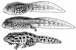
Figure 3. Pearson Scott Foresman, Public domain, via Wikimedia Commons

The question we addressed: metamorphosis of Anuran tadpoles to adults (frogs) likely involves increased metabolic demands, demands that may exceed simple allometric predictions based on increase in body size during development. Thus, we predicted that mass-specific metabolic rate for metamorphic frogs would exceed mass-specific metabolism of pre-metamorphic frogs.

M. Dohm unpublished results from my undergraduate days (1986!), you’ll find this simple data set at the bottom of this page (scroll or click here). For simplicity, we grouped all tadpoles between stages 35 and 38 as Stage I and all tadpoles between 39 and 44 as stage II. No tadpoles who completed metamorphosis were included in the dataset. It shouldn’t surprise you — with such a small sample size, the project lacked power to test the hypothesis, but many such studies, it’s worth looking at in the case anyway because the prevailing sentiment is that the metabolic cost of metamorphosis is significant — in other words, we expect a large effect size — and remains an ongoing research effort (see Burraco et al 2019).

You should confirm your self, but the slope of the regression equation of oxygen consumption (ml O₂/hour) on body mass (g) was 444.95 (with SE = 65.89). Plot of data shown in Figure 4.

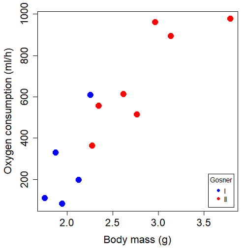
Oxygen consumption of tadpoles by body weight

Figure 4. Scatterplot of oxygen consumption by tadpoles (blue: Gosner developmental stage I [35 – 38]; red: Gosner developmental stage II [39 – 44]), vs body mass (g).

The project looked at whether metabolism as measured by oxygen consumption was consistent across two developmental stages. Metamorphosis in frogs and other amphibians represents profound reorganization of the organism as the tadpole moves from water to air. Thus, we would predict some cost as evidenced by change in metabolism associated with later stages of development. Figure 5 shows a box plot of tadpole oxygen consumption by Gosner (1960) developmental stage.

boxplot oxygen consumption of tadploes by developmental stage

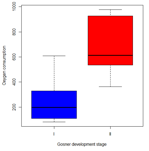
Figure 5. Boxplot of oxygen consumption by Gosner developmental stages (blue: stage I; red: stage 2).

Looking at Figure 4 we see a trend consistent with our prediction; developmental stage may be associated with increased metabolism. However, older tadpoles also tend to be larger, and the plot in Figure 4 does not account for that. Thus, body mass is a confounding variable in this example. There are several options for analysis here (e.g., ANCOVA), but one way to view this is to compare the slopes for the two developmental stages. While this test does not compare the means, it does ask a related question: is there evidence of change in rate of oxygen consumption relative to body size between the two developmental stages? The assumption that the slopes are equal is a necessary step for conducting the ANCOVA, which we describe in Chapter 17.6.

So, divide the data set into two groups by developmental stage (12 tadpoles could be assigned to one of two developmental stages; one tadpole was at a lower Gosner stage than the others and so is dropped from the subset).

Gosner stage I (stages 35 – 39)

Body mass	$\dot{V}O_{2}$
1.76	109.41
1.88	329.06
1.95	82.35
2.13	198
2.26	607.7

Gosner stage II (stage 40 – 44)

Body mass	$\dot{V}O_{2}$
2.28	362.71
2.35	556.6
2.62	612.93
2.77	514.02
2.97	961.01
3.14	892.41
3.79	976.97

The slopes and standard errors were

	Gosner Stage I	Gosner stage II
slope	750.0	399.9
standard error of slope	444.6	111.2

Are the two slopes equal?

Looking at the table, we would say, no. slopes look different (750 vs 399.9). However, the errors are large and, given this is a small data set, we need to test statistically; are the slopes indistinguishable (Ho: b_I = b_II), where b_I is the slope for the Gosner Stage I subset and b_II is the slope for the Gosner Stage II subset?

To use our tests discussed above, we need sum of squared X values for Gosner Stage I and sum of squared for Gosner stage II results. We can get these from the ANOVA tables. Recall that after applying

ANOVA regression Gosner Stage I, R work

Anova(gosI.1, type="II")
Anova Table (Type II tests)

Response: VO2
            Sum Sq   Df    F value   Pr(>F)
Body.mass    89385    1     2.8461   0.1902
Residuals    94220    3

ANOVA regression Gosner Stage II

Anova(gosII.1, type="II")
Anova Table (Type II tests)

Response: VO2
             Sum Sq    Df   F value  Pr(>F) 
Body.mass    258398     1    12.935  0.0156 *
Residuals     99882     5

Rcmdr: Models – Compare model coefficients..

compareCoefs(gosI.1, gosII.1)
Calls:
1: lm(formula = VO2 ~ Body.mass, data = gosI)
2: lm(formula = VO2 ~ Body.mass, data = gosII)

            Model 1    Model 2
(Intercept)   -1232       -441
SE              891        321

Body.mass       750        400
SE              445        111

SSgosnerI = 89385

SSgosnerII = 258398

We also need the residual Mean Squares (SSresid/DF resid) from the ANOVA tables

MSgosnerI = 94220/3 = 31406.67

MSgosnerII = 99882/5 = 19976.4

[under construction] Therefore, the pooled residual MS (s²_x.y)_p = nnn and the pooled SE of the difference s_b1-b2 = nnn using the formulas above.

Now, we plug in the values I can get a t-test = (750 – 444.6)/nnn = nnn

The DF for this t-test are n1 + n2 – 4 = 4 + 6 – 4 = 6.

Using Table of Student’s t distribution (Appendix), I find the two-tailed critical value for t at alpha = 5% with DF = 6 is equal to 3.758. Since nn >> 3.758, we conclude that the two slopes are statistically different and P < 0.001 that the null hypothesis (Ho: b_w = b_all) was true. (edit: fix nn).

Questions

Metabolic rates like oxygen consumption over time are well-known examples of allometric relationships. That is, many biological variables (e.g., $\dot{V}O_{2}$ is related as a · M^b, where M is body mass, b is scaling exponent (the slope!), and a is a constant (the intercept!)), and best evaluated on log-log scale. Redo the linear regression of oxygen consumption vs. body mass for the tadpoles, but this time, apply log10-transform to VO2 and to Body.mass. For example

Data in this page, bird matings

Body mass	Matings
29	0
29	2
29	4
32	4
32	2
35	6
36	3
38	3
38	5
38	8
40	6

Data in this page, Oxygen consumption, $\dot{V}O_{2}$ , of Anuran tadpoles

Gosner	Body mass	VO2
NA	1.46	170.91
I	1.76	109.41
I	1.88	329.06
I	1.95	82.35
I	2.13	198
II	2.28	362.71
I	2.26	607.7
II	2.35	556.6
II	2.62	612.93
II	2.77	514.02
II	2.97	961.01
II	3.14	892.41
II	3.79	976.97

Gosner refers to Gosner (1960), who developed a criteria for judging metamorphosis staging.