9.2 – Chi-square contingency tables
 from a, b, c, and d 2X2 table format formula
 effect size
Introduction
This page covers a lot of ground to extend our discussion of implementations of the chi-square test to experimental data and introduces several related statistics, including a correlation coefficient for categorical data and an introduction to agreement and reliability measurement statistics.
We begin with contingency tables.
We just completed a discussion about goodness of fit tests, inferences on categorical traits for which a theoretical distribution or expectation is available. We offered Mendelian ratios as an example in which theory provides clear-cut expectations for the distribution of phenotypes in the F2 offspring generation. This is an extrinsic model — theory external to the study guides in the calculation of expected values — and it reflects a common analytical task in epidemiology.
But for many other kinds of categorical outcomes, no theory is available. Today, most of us accept the link between tobacco cigarette smoking and lung cancer. The evidence for this link was reported in many studies, some better designed than others.
Consider the famous Doll and Hill (1950) report on smoking and lung cancer. They reported (Table IV Doll and Hill 1950), for men with lung cancer, only two out of 649 were non-smokers. In comparison, 27 case-control patients (ie, patients in the hospital but with other ailments, not lung cancer) were nonsmokers, but 622 were smokers (Table 1).
Table 1. Doll and Hill (1950).
| Smokers | Non-smokers | |
| Lung cancer | 647 | 2 |
| Case controls, no lung cancer | 622 | 27 |
A more recent example from the study of the efficacy of St John’s Wort (Hypericum perforatum) as a treatment for major depression (Shelton et al 2001, Apaydin et al. 2016). Of patients who received St. John’s Wort over 8 weeks, 14 were deemed improved while 98 did not improve. In contrast 5 patients who received the placebo were deemed improved while 102 did not improve (Table 2).
Table 2. St. John’s Wort and depression
| Improved | Not improved | |
| St. John’s Wort | 14 | 98 |
| Placebo | 5 | 102 |
Note 1: The St. John’s Wort problem is precisely a the time to remind any reader of Mike’s Biostatistics Book: under no circumstances is medical advice implied from my presentation. From the National Center for Complementary and Integrative Medicine: “It has been clearly shown that St. John’s wort can interact in dangerous, sometimes life-threatening ways with a variety of medicines.”
These kinds of problems are direct extensions of our risk analysis work in Chapter 7. Now, instead of simply describing the differences between case and control groups by Relative Risk Reduction or odds ratios, we instruct how to do inference on the risk analysis problems.
Thus, faced with absence of coherent theory as guide, the data themselves can be used (intrinsic model), and at least for now, we can employ the  test.
test.
Note 2: The preferred analysis is to use a logistic regression approach, Chapter 18.3, because additional covariates can be included in the model.
In this lesson we will learn how to extend the analyses of categorical data to cases where we do not have a prior expectation — we use the data to generate the tests of hypotheses. This would be an intrinsic model. One of the most common two-variable categorical analysis involves 2X2 contingency tables. We may have one variable that is the treatment variable and the second variable is the outcome variable. Some examples provided in Table 3.
Table 3. Some examples of treatment and outcome variables suitable for contingency table analysis.
| Treatment Variable and Levels | Outcome Variable(s) | Reference |
| Lead exposure
Levels: Low, Medium, High |
Intelligence and development | Bellinger et al 1987 |
| Wood preservatives
Levels: Borates vs. Chromated Copper Arsenate |
Effectiveness as fungicide | Hrastnik et al 2013 |
| Antidepressants
Levels: St. John’s Wort, conventional antidepressants, placebo |
Depression relief | Linde et al 2008 |
| Coral reefs
Levels: Protected vs Unprotected |
Fish community structure | Guidetti 2006 |
| Aspirin therapy
Levels: low dose vs none |
Cancer incidence in women | Cook et al 2013 |
| Aspirin therapy
Levels: low dose vs none |
Cancer mortality in women | Cook et al 2013 |
Table 4 were examples of published studies returned from a quick PubMed search; there are many examples (meta-analysis opportunities!). However, while they all can be analyzed by contingency tables analysis, they are not exactly the same. In some cases, the treatments are fixed effects, where the researcher selects the levels of the treatments (see Ch12.3 and Ch14.3 for discussion about fixed vs random effects in experimental design).
In other cases, each of these treatment variables need not be actual treatments (in the sense that an experiment was conducted), but it may be easier to think about these as types of experiments. These types of experiments can be distinguished by how the sampling from the reference population were conducted. Before we move on to our main purpose, to discuss how to calculate contingency tables, I wanted to provide some experimental design context by introducing two kinds of sampling (Chapter 5.5).
Our first kind of sampling scheme is called unrestricted sampling. In unrestricted sampling, you collect as many subjects (observations) as possible, then assign subjects to groups. A common approach would be to sample with a grand total in mind; for example, your grant is limited and so you only have enough money to make 1000 copies of your survey and you therefore approach 1000 people. If you categorize the subjects into just two categories (eg, Liberal, Conservative), then you have a binomial sample. If instead you classify the subjects a number of variables, eg, Liberal or Conservative, Education levels, income levels, homeowners or renters, etc., then this approach is called multinomial sampling. The point in either case is that you have just utilized a multinomial sampling approach. The aim is to classify your subjects to their appropriate groups after you have collected the sample.
Logically what must follow unrestricted sampling would be restricted sampling. Sampling would be conducted with one set of “marginal totals” fixed. Margins refers to either the row totals or to the column totals. The sampling scheme is referred to as compound multinomial. The important distinction from the other two types is that the number of individuals in one of the categories is fixed ahead of time. For example, in order to determine if smoking influences respiratory health, you approach as many people as possible to obtain 100 smokers.
The contingency table analysis
We introduced the 2×2 contingency table (Table 4) in Chapter 7.
Table 4. 2X2 contingency table
| Outcome |
|||
| Exposure or Treatment group | Yes | No | Marginal total |
| Exposure (Treatment) | a | b | Row1 = a + b |
| Nonexposure (Control) | c | d | Row2 = c + d |
| Marginal total | Column1 = a + c |
Column2 = a + c |
N |
Contingency tables are all of the form (Table 5)
Table 5. Basic format of a 2X2 table
| Outcome 1 | Outcome 2 | |
| Treatment 1 | Yes | No |
| Treatment 2 | Yes | No |
Regardless of how the sampling occurred, the analysis of the contingency table is the same; mechanically, we have a chi-square type of problem. In both contingency table and the “goodness of fit” Chi-Square analyses the data types are discrete categories. The difference between GOF and contingency table problems is that we have no theory or external model to tell us about what to expect. Thus, we calculate expected values and the degrees of freedom differently in contingency table problems. To learn about how to perform contingency tables we will work through an example, first the long way, and then using a formula and the a, b, c, and d 2X2 table format. Of course, R can easily do contingency tables calculations for us.
Doctors noticed that a new form of Hepatitis (HG, now referred to as GB virus C), was common in some HIV+ populations (Xiang et al 2001). Accompanying the co-infection, doctors also observed an inverse relationship between HG loads and HIV viral loads: patients with high HG titers often had low HIV levels. Thus, the question was whether co-infection alters the outcome of patients with HIV — do HIV patients co-infected with this HG progress to AIDS and mortality at rates different from non-infected HIV patients? I’ve represented the Xiang et al (2001) data in Table 6.
Table 6. Progression of AIDS for patients co-infected with HG [GB virus C], Xiang et al data (2001)
| Lived | Died | Row totals | |
| HG+ | 103 | 41 | 144 |
| HG- | 95 | 123 | 218 |
| Column totals | 198 | 164 | 362 |
Note 3: HG virus is no longer called a hepatitis virus, but instead is referred to as GB virus C, which, like hepatitis viruses, is in the Flaviviridae virus family. For more about the GB virus C, see review article by Bhattarai and Stapleton (2012).
Our question was: Do HIV patients co-infected with this HG progress to AIDS and mortality at rates different from non-infected HIV patients? A typical approach to analyze such data sets is to view the data as discrete categories and analyze with a contingency table. So we proceed.
Setup the table for analysis
Rules of contingency tables (see Kroonenberg and Verbeek 2018). What follows is a detailed walk through setting up and interpreting a 2X2 table. Note that I maintain our a, b, c, d cell order, with row 1 referencing subjects exposed or part of treatment group and row 2 referencing subjects not exposed (or part of the control group), as introduced in Chapter 7.
The Hepatitis G data from Xiang et al 2001 data, arranged in 2X2 format (Table 7).
Table 7. Format of 2X2 table Xiang et al (2001) dataset.
| Lived | Died | Row totals | |
| HG+ | a | b | a + b |
| HG- | c | d | c + d |
| Column totals | a + c | b + d | N |
The data are placed into the cells labeled a, b, c, and d.
Cell a : The number of HIV+ individuals infected with HG that lived beyond the end of the study.
Cell b : The number of HIV+ individuals infected with HG that died during the study.
Cell c : The number of HIV+ individuals not infected with HG that lived.
Cell d : The number of HIV+ individuals not infected with HG that died.
This is a contingency table because the probability of living or dying for these patients may have been contingent on coinfection with hepatitis G.
State the examined hypotheses
HO: There is NO association between the probability of living and coinfection with hepatitis G.
For a contingency table this means that there should be the same proportion of individuals with and without hepatitis G that either lived or died (1:1:1:1).
Now, compute the Expected Values in the Four cells (a, b, c, d)
- Calculate the Expected Proportion of Individuals that lived in Entire Sample:
Column 1 Total / Total = Expected Proportion of those that lived beyond the study. - Calculate Expected Proportion of Individuals that died in Entire Sample:
Column 2 Total / Total = Expected Proportion that died during the study. - Calculate the Expected Proportion of Individuals that lived and were HG+
Expected Proportion of living (step 1 above) x Row 1 Total = Expected For Cell A. - Calculate the Expected Proportion of Individuals that died and were HG+
Expected Proportion died x Row 1 Total = Expected For Cell B - Calculate the Expected Proportion of surviving individuals that were HG-
Expected Proportion lived x Row 2 Total = Expected For Cell C - Calculate the Expected Proportion of individuals that died that were HG-
Expected Proportion that died x Row 2 Total = Expected For Cell D
Yes, this can get a bit repetitive! But, we are now done — remember, we’re working through this to review how the intrinsic model is applied to obtain expected values.
To summarize what we’ve done so far, we now have
Observations arranged in a 2X2 table
Calculated the expected proportions, ie, the Expected values under the Null Hypothesis.
Now, we proceed to conduct the chi-square test of the null hypothesis — The observed values may differ from these expected values, meaning that the Null Hypothesis is False.
Table 8. Copy Table 6 data set
| Lived | Died | Row totals | |
| HG+ | 103 | 41 | 144 |
| HG- | 95 | 123 | 218 |
| Column totals | 198 | 164 | 362 |
Get the Expected Values
- Calculate the Expected Proportion of Individuals that lived in Entire Sample:
Column 1 Total (198) / Total (362) = 0.5470 - Calculate Expected Proportion of Individuals that died in Entire Sample:
Column 2 Total (164) / Total (362) = 0.4530 - Calculate the Expected Proportion of Individuals that lived and were HG+
Expected Proportion of living (0.547) x Row 1 Total (218) = Cell A = 119.25 - Calculate the Expected Proportion of Individuals that died and were HG+
Expected Proportion died (0.453) x Row 1 Total (218) = Cell B = 98.75. - Calculate the Expected Proportion of surviving individuals that were HG-
Expected Proportion lived (0.547) x Row 2 Total (144) = Cell C = 78.768 - Calculate the Expected Proportion of individuals that died that were HG-
Expected Proportion that died 0(.453) X Row 2 Total = Cell D = 65.232
Thus, we have (Table 9)
Table 9. Expected values for Xiang et al (2001) data set (Table 6 and Table 8)
| Lived | Died | Row totals | |
| HG+ | 78.768 | 65.232 | 144 |
| HG- | 119.25 | 98.75 | 218 |
| Column totals | 198 | 164 | 362 |
Now we are ready to calculate the Chi-Square Value
Recall the formula for the chi-square test

Table 10. Worked contingency table for Xiang et al (2001) data set (Table 6 and Table 8)
| Cell |  |
|
| a | (103 – 87.768)2 = 78.768 | 7.4547 |
| b | (41 – 65.232)2 = 65.232 | 9.002 |
| c | (95 – 119.25)2 = 119.25 | 4.93134 |
| d | (123 – 98.75)2 = 98.75 | 5.95506 |
 |
27.3452 |
Adding all the parts we have the chi-square test statistic  . To proceed with the inference, we test using the chi-square distribution.
Determine the Critical Value of  test and evaluate the null hypothesis
Now recall that we can get the critical value of this test in one of two (related!) ways. One, we could run this through our statistical software and get the p-value, the probability of our result and the null hypothesis is true. Second, we look up the critical value from an appropriate statistical table. Here, we present option 2.
We need the Type I error rate α and calculate the degrees of freedom for the problem. By convention, we set α = 0.05. Degrees of freedom for contingency table is calculated as
Degrees of Freedom = (# rows – 1) x (# columns – 1)
and for our example → DF = (2 – 1) x (2 – 1) = 1.
Note. How did we get the 1 degree of freedom? Aren’t there 4 categories and shouldn’t we therefore have k – 1 = 3 df? We do have four categories, yes, but the categories are not independent. We need to take this into account when we evaluate the test and this lack of independence is accounted for by the loss of degrees of freedom.
What exactly is not independent about our study?
-
- The total number of observations is set in advance from the data collection.
- We also have the column and row totals set in advance. The number of HIV individuals with or without Hepatitis G infection was determined at the beginning of the experiment. The number of individuals that lived or died was also determined before we we conducted the test.
- Then the first cell (let us make that cell A) can still vary anywhere from 0 to N i (sample size of the first drug).
- Once the first cell (A) is determined then the next cell in that row (B) will have to add up to N i.
- Also the other cell in the same column as the first cell (C) must add up to the Column 1 Total.
- Lastly, the last cell (D) must have the Row 1 Total add up to the correct number.
All this translates into there being only one cell that is FREE TO VARY, hence, only one degree of freedom.
Get the Critical Value from a chi-square distribution table: For our example, look up the critical value for DF = 1, α = 0.05, you should get 3.841. The 3.841 is the value of the chi-square we would expect at 5% and the null hypothesis is in fact true condition in the population.
Once we obtain the critical value we simply use the previous statement regarding the probability of the Null Hypothesis being TRUE. We Reject the Null Hypothesis when the calculated test statistic is greater than the Critical Value. We Accept the Null Hypothesis when the calculated is less than the Critical Value. In our example we got 27.3452 for our calculated test statistic, thus we reject the null hypothesis and conclude, that, at least for the sample in this study, there was an association between the probability of patients living past the study period and the presence of hepatitis G.
from a, b, c, and d 2X2 table format formula
If a hand calculation is required, a simpler formula to use is

where N is the sum of all observations in the table, r1 and r2 are the marginal row totals, and c1 and c2 are the marginal column totals from the 2×2 contingency table (eg, Table 4). If you are tempted to try this in a spreadsheet, and assuming your entries for a, b, c, d, and N look like Table 11, then a straightforward interpretation requires referencing five spreadsheet cells no less than 13 times! Not to mention a separate call to the distribution to calculate the p-value (one tailed test).
Note 4: This formulation was provided as equation 1 in Yates 1984 (referred to in Serra 2018), but is likely found in the earlier papers on dating back to Pearson.
Table 11. Example spreadsheet with formulas for odds ratio (OR), Pearson’s , and p-value from distribution.
| A | B | C | D | E | F | G | |
| 1 | |||||||
| 2 | a | 103 | OR | =( 2*5)/(3*4) 2*5)/(3*4) |
|||
| 3 | b | 41 | |||||
| 4 | c | 95 | |||||
| 5 | d | 123 | chisq, p | =(((2*5-3*4)^2)*6)/ (SUM( 2:3)*SUM(4:5)*SUM( 2,4)*SUM(3,5)) |
=CHIDIST(F5,1) | ||
| 6 | N | 632 |
Now, let’s see how easy this is to do in R.
effect size
Inference on hypotheses about association, there’s statistical significance — evaluate p-value compared to Type I error, eg, 5% — and then there’s biological importance, the strength of the association. The concept of effect size is an attempt to communicate the likely importance of a result. Several statistics are available to communicate effect size: for that’s φ, phi for the φ (phi) coefficient.

where N is the total. Phi for our example is

R code
sqrt(27.3452/362)
and R returns
[1] 0.274844
Effect size statistics typically range from 0 to 1; Cohen (1992) suggested the following interpretation
Table 12. Cohen’s interpretation of d values.
| Effect size | Interpretation |
| < 0.2 | Small, weak effect |
| 0.5 | Moderate effect |
| > 0.8 | Large effect |
For our example,  effect size of the association between co-infection with GB virus C and mortality was weak in the patients with HIV infection. The function
 phi() in psych package will calculate phi coefficient from a 2X2 table.
Agreement, kappa, and inter-rater reliability
I imagine by now you have made the leap — can we use the contingency table to assess agreement between (inter-) two judges (raters) who evaluate the same object? A naive approach would be to calculate simple agreement, the percent of objects in the list of items evaluated for which both judges agree (concur). For a binomial Yes or No, then agreement (concordance) occurs when both judges report “Yes,” or both report “No,” displayed on the main diagonal of the 2X2 table. The other possible combinations (Yes vs No and No vs Yes) are disagreement (discordance) and would be displayed on the off-diagonal of the 2X2 matrix.
Unfortunately, simple agreement, while intuitive, cannot discriminate between true agreement and agreement by chance. Cohen’s kappa (Cohen 1960, McHugh 2012) is used to assess agreement, aka inter-rater reliability, for binomial and nominal data types for two judges (raters). Cohen’s 1960 paper has been enormously impactful, with more than 53K citations (Google Scholar, Fall 2024), and spawned a number of additional measures of agreement, eg, weighted kappa for more than binomial levels, Fleiss kappa for three or more raters, ICC for ratio scale, discussed in Ch12.3). It’s beyond the scope of this text to review the context of such terms as agreement, and reliability, for just two terms used to evaluate results from two independent observers of the “same” event or object, and leave that to the reader to confirm how to report such endeavors.
Off we go. Cohen’s kappa is defined as

where po is the proportion in agreement and pc is proportion of agreement expected by chance. Essentially, then, interpretable kappa values fall between 0 and 1 (0% to 100%); negative kappa estimates are possible. Cohen (1960) noted that for kappa to equal 1, the off diagonal elements would all have to be zero.
Cohen provided an estimate of the standard error for kappa as

and 95% confidence intervals are then  .
.
Here, we review calculation of simple agreement and Cohen’s kappa, with just the two levels. Both simple agreement and Cohen’s kappa (κ), are available in R via the icc package. Cohen’s kappa is also available in the psych package, with the cohen.kappa() function providing a confidence interval estimate directly.
Note 5: Base R includes the function kappa(), but that returns an estimate for the condition number of the matrix, or how close to singular the matrix solution may be, ie, determinant is zero and its inverse is unavailable.
Use of both is illustrated here with a simulated coin toss example modified from a nice 2018 summary of Cohen’s kappa at r-bloggers. The R code
library(irr)
# simulate some data
N = 24
flips1 <- rbinom(n = N, size = 1, prob = 0.5)
flips2 <- rbinom(n = N, size = 1, prob = 0.5)
coins<-cbind(flips1, flips2)
Confirm the data set.
head(coins)
flips1 flips2
[1,] 0 1
[2,] 1 0
[3,] 1 0
[4,] 1 1
[5,] 0 0
[6,] 1 0
and create a 2X2 table.
I stacked the data
head(StackedCoin)
Side Coins    HT
1 0 flips1 tails
2 1 flips1 heads
3 1 flips1 heads
4 1 flips1 heads
5 0 flips1 tails
6 1 flips1 heads
then created a simple 2×2 table (see Note 6 below for a simple explanation for why “.Table” as a named object).
.Table <- xtabs(~Coins+HT, data=StackedCoin)
Table 13. coins as 2X2 table.
| tails | heads | |
| flips1 | 10 | 14 |
| flips2 | 14 | 10 |
We can calculate the phi coefficient for Table 13.
phi(.Table, digits = 3)
[1] -0.167
and would conclude no correlation between the two sets of coin tosses.
Now, agreement statistics. Both agree() and kappa2() expect an unstacked (wide) data format. It’s not necessary, but we’ll call a value of 1 as “heads up” and a value of 0 as “tails up” of the tossed coin.
Next, simple agreement.
agree(coins, tolerance=0)
R returns
Subjects = 24
Raters = 2
%-agree = 41.7
Now, a proper agreement statistic.
kappa2(coins)
and R returns
Subjects = 24
Kappa = -0.135
z = -0.7
p-value = 0.484
Results with psych:cohen.kappa, which provides the 95% confidence interval as default output.
Cohen Kappa and Weighted Kappa correlation coefficients and confidence boundaries
                 lower estimate upper
unweighted kappa -0.51    -0.14  0.24
weighted kappa   -0.51    -0.14  0.24
Number of subjects = 24
By chance, the two independent toss of 24 coins had 10 rows of “agreement” (H:H or T:T), simply due to chance. However, results of kappa find no agreement between the two sets of coin tosses.
In summary, we see that simple agreement and the kappa statistic don’t return similar results. Percent agreement reported 41%, whereas kappa was zero. We know percent agreement can’t reflect anything in the coin toss case because each toss is independent from the next. We’ll have you explore repeated trials of coin tosses to help convince you that simple agreement is not a reliable measure of agreement (see question 6 below).
Interpreting agreement values is not straightforward, and some argue agreement statistics should be avoided in favor of disagreement measures (for example, see discussion in Pontius and Millones 2011). Cohen suggested (Table 14)
Table 14. Landis and Koch’s (1977) interpretation of Cohen’s kappa.
| Cohen’s kappa | Agreement? |
| < 0 | none |
| 0.01 — 0.20 | slight |
| 0.21 — 0.40 | fair |
| 0.41 — 0.60 | moderate |
| 0.61 — 0.80 | substantial |
| 0.81 — 1 | nearly perfect |
Note 6: Wikipedia page for Cohen’s kappa suggests that this interpretation began with the Landis and Koch 1997 paper in the journal Biometrics. I haven’t confirmed this — regardless, this paper is also highly influential, with more than 89K citations (Fall 2024).
Even a cursory look at Table 14 should lead to questions about scenarios in which a range of agreement “substantial” would provide little comfort about the agreement between the judges or the reliability of the instrument used, for example forensic cases or histology of tissue biopsies.
Contingency table analyses in Rcmdr
Assuming you have already summarized the data, you can enter the data directly in the Rcmdr contingency table form. If your data are not summarized, then you would use Rcmdr's Two-way table… for this. We will proceed under the assumption that you have already obtained the frequencies for each cell in the table.
Rcmdr: Statistics → Contingency tables → Enter and analyze two-way table…
Here you can tell R how many rows and how many columns (Fig 1).
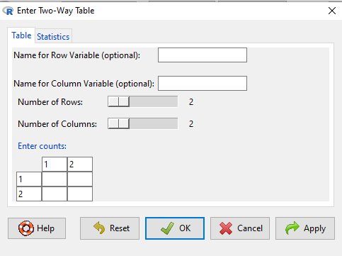
Figure 1. Screenshot R Commander menu for 2X2 data entry with counts.
The default is a 2X2 table. For larger tables, use the sliders to increase the number of rows, columns, or both.
Next, enter the counts. You can edit every cell in this table, including the headers. In the next panel, I will show you the data entry and options. The actual calculation of the test statistic is done when you select the “Chi-square test of independence” check-box (Fig 2).
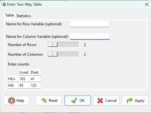
Figure 2. Display of Xiang et al data entered into R Commander menu.
After entering the data, click on the Statistics tab (Fig 3).
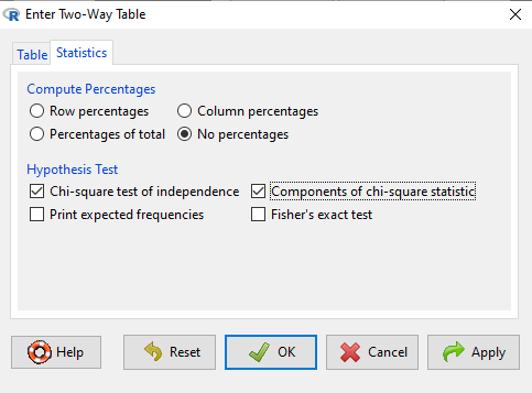
Figure 3. Screenshot Statistics options for contingency table.
If you also select “Components of chi-square statistic” option, then R will show you the contributions of each cell (O-E) towards the chi-square test statistic value. This is helpful to determine if rejection of the null is due to a subset of the categories, and it also forms the basis of the heterogeneity tests, a subject we will pick up in the next section.
Here’s the R output from R Commander. Note the “2, 2, byrow=TRUE” instructions (check out R help to confirm what
.Table <- matrix(c(103,41,95,123), 2, 2, byrow=TRUE)
dimnames(.Table) <- list("rows"=c("HG+", "HG-"), "columns"=c("Lived", "Died"))

.Table # Counts
     columns
rows Lived Died
 HG+   103   41
 HG-   95   123

.Test <- chisq.test(.Table, correct=FALSE)
.Test

Pearson's Chi-squared test

data: .Table
X-squared = 27.339, df = 1, p-value = 0.0000001708

round(.Test$residuals^2, 2) # Chi-square Components
    columns
rows Lived Died
HG+   7.46 9.00
HG-   4.93 5.95

remove(.Test)
remove(.Table)
end R output.
Note 7: R Commander often cleans up after itself by removing objects like .Test and .Table. This is not necessary for the code to work, but does make it easier for you to go back and modify the code without worrying about confusing objects.
Lots of output, take a deep breath and remember… The minimum output we need to look at is… (Table 15)?
Table 15. Minimally expected outcome for report from a statistical test.
| Value of the test statistic | 27.339 |
| Degrees of freedom | 1 |
| p-value | 0.0000001708 |
We can see that the p-value 1.7-7 is much less than Type 1 α = 0.05, thus, by our decision criterion we reject the null hypothesis (provisionally of course, as science goes).
Note 7: Simple enough to get R to report numbers as you need. For example, R code
myNumber = 0.0000001708
format(myNumber, scientific = TRUE, digits=2)
returns
[1] "1.7e-07"
Questions
- Instead of R Commander, try the contingency table problem in R directly.
myData <- matrix(c(103,41,95,123))
chisq.test(myData)
Is this the correct
contingency table analysis? Why or why not? - For many years National Football League games that ended in ties went to “sudden death,” where the winner was determined by the first score in the extra period of play, regardless of whether or not the other team got an opportunity to possess the ball on offense. Thus, in more than 100 games (140), the team that won the coin toss and therefore got the ball first in overtime, won the game following either a kicked field goal or after a touchdown was scored. In 337 other games under this system, the outcome was not determined by who got the ball first. Many complained that the “sudden death” format was unfair and in 2013 the NFL changed its overtime rules. Beginning 2014 season, both teams got a chance to possess the ball in overtime, unless the team that won the coin toss also went on to score a touchdown at which time that team would be declared the winner. In this new era of over-time rules ten teams that won the coin toss went on to score a touchdown in their first possession and therefore win the game, whereas in 54 other overtime games, the outcome was decided after both teams had a chance on offense (data as of 1 December 2015). These data may be summarized in the table
First possession win? Yes No Coin flip years 140 337 New era 10 54 A. What is the null hypothesis?
B. Which is more appropriate: to calculate an odds ratio or to calculate an RRR?
C. This is a contingency table problem. Explain why
D. Conduct the test of the null hypothesis.
E. What is the value of the test statistic? Degrees of freedom? P-value?
F. Evaluate the results of your analysis — do you accept or reject the null hypothesis? - Return to the Doll and Hill (1950) data: 2 men with lung cancer were nonsmokers, 647 men with lung cancer were cigarette smokers. In comparison, 27 case-control patients (ie, patients in the hospital but with other ailments, not lung cancer) were nonsmokers, but 622 were cigarette smokers.
A. What is the null hypothesis?
B. Which is more appropriate: to calculate an odds ratio or to calculate an RRR?
C. This is a contingency table problem. Explain why
D. Conduct the test of the null hypothesis.
E. What is the value of the test statistic? Degrees of freedom? P-value?
F. Evaluate the results of your analysis — do you accept or reject the null hypothesis? - A more recent example from the study of the efficacy of St John’s Wort as a treatment for major depression (Shelton et al 2001). Of patients who received St. John’s Wort over 8 weeks, 14 were deemed improved while 98 did not improve. In contrast 5 patients who received the placebo were deemed improved while 102 did not improve.
A. What is the null hypothesis?
B. Which is more appropriate: to calculate an odds ratio or to calculate an RRR?
C. This is a contingency table problem. Explain why
D. Conduct the test of the null hypothesis.
E. What is the value of the test statistic? Degrees of freedom? P-value?
F. Evaluate the results of your analysis — do you accept or reject the null hypothesis? - Return to the coin toss simulation and repeat comparisons between simple agreement and Cohen’s kappa for different values of N. Do you see any trend(s) for the two measures as sample size increases or decreases?
- Repeat the coin toss simulation for N = 24 up to five times, each time calculate simple agreement and Cohen’s kappa. Provide a table of your five results plus the example, and generalize simple agreement vs Cohen’s kappa as a reliable measure of agreement. Hint: you may want to use Descriptive statistics to help make your case.
Quiz Chapter 9.2
Chi-square contingency tables