20.11 – Plot a Newick tree
Introduction
The phrase “paradigm shift”, attributed to Kuhn (1962, see Wikipedia), may be well-worn and even abused today (Naughton 2012), but the shift in thinking from essential types and group thinking (essentialism) to viewing species as varying individuals in populations (populating thinking) revolutionized biology (O’Hara 1997, Sandvik 2008). Tree thinking is the manifestation of Charles Darwin’s “descent with modification” metaphor (Gregory 2008). Thus, every biology student should have ability to work with, and interpret, phylogenetic trees (tree thinking). The subject of creating and working with phylogenetic graphs is complicated with an extensive library. A good review is available from Holder and Lewis (2003) and readers should know Felsenstein’s book (2004).
Here, I include a modest, incomplete primer on working with trees in R.
- Loading the tree file
- Change tip names
- Write tip names to a text file
- Plot the tree as phylogram or cladogram
- Get node labels
- Re-root the tree
- Write a tree to a file
I assume that the student already has a set of species or other taxa, gathered sequences (DNA or protein), aligned the sequences, estimated gene or phylogeny tree, and wishes to view and manipulate the tree in R. While these kinds of analyses can be done with R and R packages (see Task view: Phylogenetics), other software may be better choice for the student just beginning with phylogenetic tree building (see Unipro UGENE and MEGA, for examples). If the goal is just to view a tree file, or add annotations, then I recommend the iTOL tools.
Data formats
Phylogeny and gene trees are special cases of network graphs. Newick format (Wikipedia) is a common but limited representation of the tree which uses parentheses (groupings) and commas (branching). Other formats permit additional information; examples are Nexus file (Wikipedia) and the extension of Nexus to XML, NeXML (Wikipedia), and phyloXML (Wikipedia) formats. Our example uses Newick format.
Data set
I’ll use a “time tree” for an example. Tree from timetree.org, list of species (copy/paste list to a text file, load the text file Load list of of Species, then save the tree as a Newick file).
Alligator mississippiensis
Felis catus
Bos taurus
Gallus gallus
Pan troglodytes
Canis lupus
Homo sapiens
Anolis carolinensis
Macaca mulatta
Mus musculus
Didelphis virginiana
Sus scrofa
Oryctolagus cuniculus
Rattus norvegicus
R code
Requires the ape package. Phylotools and Phytools packages provide additional handy functions. References for these packages are listed at the end of this page.
require(ape)
require(phytools)
require(phylotools)
#If tree file, then
read.tree(file="tree14.nwk")
or
tree14 <- read.tree(file.choose())
#If no tree file saved, copy the Newick data use text="", replace example tree with your Newick tree
tree14 <-read.tree(text="((Anolis_carolinensis:279.65697667,(Gallus_gallus:236.50266286,Alligator_mississippiensis:236.50266286)'14':43.15431381)'13':32.24694470,(Didelphis_virginiana:158.59758758,(((Felis_catus:54.32144118,Canis_lupus:54.32144118)'11':23.43351523,(Bos_taurus:61.96598852,Sus_scrofa:61.96598852)'10':15.78896789)'19':18.70743276,((Oryctolagus_cuniculus:82.14079889,(Rattus_norvegicus:20.88741740,Mus_musculus:20.88741740)'9':61.25338149)'22':7.68238853,(Macaca_mulatta:29.44154682,(Pan_troglodytes:6.65090500,Homo_sapiens:6.65090500)'8':22.79064182)'6':60.38164060)'30':6.63920175)'29':62.13519841)'27':153.30633379);")
#return information about the object
tree14
Output returned by R
Phylogenetic tree with 14 tips and 13 internal nodes.
Tip labels:
Anolis_carolinensis, Gallus_gallus, Alligator_mississippiensis, Didelphis_virginiana, Felis_catus, Canis_lupus, ...
Node labels:
, 13, 14, 27, 29, 19, ...
Rooted; includes branch lengths.
Change the tip names. Create a data frame with the tip labels and new tip names.
require(phylotools)
timeTreeTips <- tree14$tip.label
replaceTips <- c("Alligator", "Cat", "Chicken", "Chimpanzee", "Cow", "Dog", "Human", "Lizard", "Macaque", "Mouse", "Opossum", "Pig", "Rabbit", "Rat")
myDat <- data.frame(timeTreeTips,replaceTips)
ntree14<- sub.taxa.label(tree14,myDat)
Collect and write the tip names to a text file
#Extract tips from newick file, write to text file
require(ape)
my.tips <- sort(tree14$tip.label)
#option 1
cat(my.tips,file="outfile.txt",sep="\n")
#option 2
my_conn = file("outfile.txt")
writeLines(my.tips,my_conn)
close(my_conn)
Next, make the plot.
plot(ntree14)
Result, a simple phylogram, i.e., a tree diagram with branching patterns and branch lengths proportional to amount of character change.
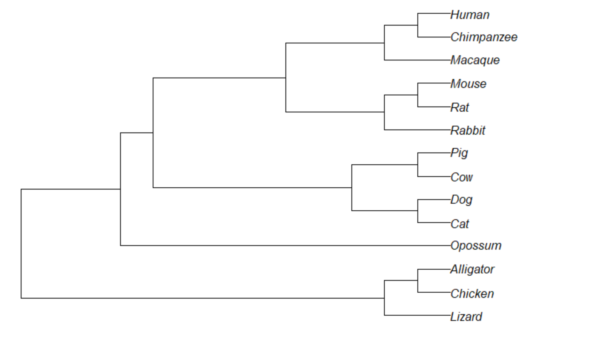
Figure 1. Phylogram plot of 14 taxa
Or, change from default “phylogram” to “cladogram” view.
plot(tree14, type="cladogram")
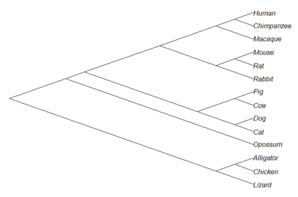
Figure 2. Cladogram view, same 14 taxa.
Note that while the tree is rooted, it’s a midpoint rooting, the default setting in Newick files. For true root based on outgroup(s), identify the nodes, then select root.
Add node labels; plot() must be run first.
nodelabels()
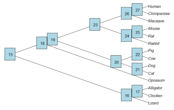
Figure 3. Plot of tree with labeled nodes.
The outgroup(s) were the reptiles (Alligator, Chicken, Lizard), so reroot at node 16.
rrTree<- root(tree14, node=16)
plot(rrTree, type="cladogram")
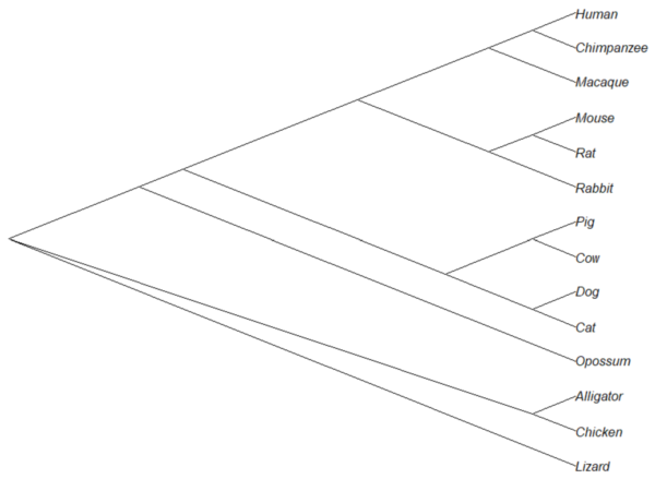
Figure 4. Re-rooted tree.
Write tree to a file
require(ape)
To export tree to Newick format
write.tree(tree14, file = "filename.nwk")
for Nexus format
write.nexus(tree14, file = "filename.nex")
Star phylogeny
Collapse the tree to a star phylogeny, an unlikely evolutionary model in which the species resulted from “… a single explosive adaptive radiation” (Felsenstein 1985). Star phylogeny is an extreme tree shape, or multifurcation (polytomy), where all tips derive from the same node (Colijn and Plazzotta 2018). This type of phylogeny can be viewed as a null model for inference (but see Bayesian “star phylogeny paradox,” cf. Kolaczkowski and Thornton 2006).
require(phytools)
ctree14 <-collapse.to.star(tree14, 15)
plot(ctree14, type="cladogram")
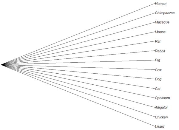
Figure 5. Star phylogeny
Under a star phylogeny model, all taxa are assumed independent of each other, in contrast to the nested hierarchical model of evolution (e.g., Fig. 4), which shows a lack of independence among the taxa. More succinctly, a fitted to uncorrected taxa comparisons may violated the assumption that errors are independent and identically distributed. Phylogenetically correct methods attempt to address the lack of independence among taxa for comparative analysis (Felsenstein 1985, Uyeda et al 2016). Biologists should know about Felsenstein’s 1985 paper. Felsenstein’s paper created a paradigm shift in how to analyze comparative datasets and has been cited more than ten thousand times (1 August 2023, Google Scholar). To put that number in context, the 1986 paper by Kary Mullis et al., which announced invention of PCR with thermally stable polymerase that has revolutionized molecular biology, has been cited 6721 times over that same period.
Additional packages of note
The R package tanggle works with the package ggtree and advantage of the ggplot2 environment. Contains many functions to work with phylogeny graphs including re-rooting and swapping nodes. The package is available from Bioconductor,
if (!requireNamespace("BiocManager", quietly = TRUE))
    install.packages("BiocManager")

BiocManager::install("tanggle")
ggtree is also a Bioconductor package, not available at CRAN.
Online viewers
Many browser-based tree viewers online, including icytree.org and iTOL tools. Additional tree viewers listed at Wikipedia.
References and suggested readings
Colijn C, Plazzotta G. A Metric on Phylogenetic Tree Shapes. Syst Biol. 2018 Jan 1;67(1):113-126.
Felsenstein, J (1985) Phylogenies and the comparative method. American Naturalist 125(1):1-15.
Felsenstein, J. (2004). Inferring phylogenies. Sunderland, MA: Sinauer associates.
Gregory, T. R. (2008). Understanding evolutionary trees. Evolution: Education and Outreach, 1(2), 121-137.
Holder, M., & Lewis, P. O. (2003). Phylogeny estimation: traditional and Bayesian approaches. Nature reviews genetics, 4(4), 275-284.
Kuhn, T. S. (1962). The structure of scientific revolutions. University of Chicago Press: Chicago.
Mullis, K., Faloona, F., Scharf, S., Saiki, R. K., Horn, G. T., & Erlich, H. (1986, January). Specific enzymatic amplification of DNA in vitro: the polymerase chain reaction. In Cold Spring Harbor symposia on quantitative biology (Vol. 51, pp. 263-273). Cold Spring Harbor Laboratory Press.
Naughton, J. (2012, August 18). Thomas Kuhn: The man who changed the way the world looked at science. The Guardian. https://www.theguardian.com/science/2012/aug/19/thomas-kuhn-structure-scientific-revolutions
O’Hara, R. J. (1997). Population thinking and tree thinking in systematics. Zoologica scripta, 26(4), 323-329.
Paradis, E. (2012) Analysis of Phylogenetics and Evolution with R (Second Edition). New York: Springer.
Paradis, E. and Schliep, K. (2019) ape 5.0: an environment for modern phylogenetics and evolutionary analyses in R. Bioinformatics, 35, 526–528.
Revell, L. J. (2012) phytools: An R package for phylogenetic comparative biology (and other things). Methods in Ecology and Evolution, 3, 217-223.
Sandvik, H. (2008). Tree thinking cannot taken for granted: challenges for teaching phylogenetics. Theory in Biosciences, 127(1), 45-51.
Uyeda, J. C., Zenil-Ferguson, R., & Pennell, M. W. (2018). Rethinking phylogenetic comparative methods. Systematic Biology, 67(6), 1091-1109.
Zhang, J., Pei, N., & Mi, X. (2012). phylotools: Phylogenetic tools for Eco-phylogenetics. R package version 0.1, 2.
Chapter 20 contents
- Additional topics
- Area under the curve
- Peak detection
- Baseline correction
- Surveys
- Time series
- Dimensional analysis
- Estimating population size
- Diversity indexes
- Survival analysis
- Growth equations and dose response calculations
- Plot a Newick tree
- Phylogenetically independent contrasts
- How to get the distances from a distance tree
- Binary classification
- Meta-analysis