18 – Multiple Linear Regression
Introduction
This is the second part of our discussion about general linear models. In this chapter we extend linear regression from one (Chapter 17) to many predictor variables. We also introduce logistic regression, which uses logistic function to model binary outcome variables. Extensions to address ordinal outcome variables are also presented. We conclude with a discussion of model selection, which applies to models with two or more predictor variables.
For linear regression models with multiple predictors, in addition to our LINE assumptions, we add the assumption of no multicollinearity. That is, we assume our predictor variables are not themselves correlated.
Rcmdr and R have multiple ways to analyze linear regression models; we will continue to emphasize the general linear model approach, which allow us to handle continuous and categorical predictor variables.
Practical aspects of model diagnostics were presented in Chapter 17; these rules apply for multiple predictor variable models. Regression and correlation (Chapter 16) both test linear hypotheses: we state that the relationship between two variables is linear (the alternative hypothesis) or it is not (the null hypothesis). The difference? Correlation is a test of association (are variables correlated, we ask?), but are not tests of causation: we do not imply that one variable causes another to vary, even if the correlation between the two variables is large and positive, for example. Correlations are used in statistics on data sets not collected from explicit experimental designs incorporated to test specific hypotheses of cause and effect. Regression is to cause and effect as correlation is to association. Regression, ANOVA, and other general linear models are designed to permit the statistician to control for the effects of confounding variables provided the causal variables themselves are uncorrelated.
Models
Chapter 17 covered the simple linear model

Chapter 18 covers multiple regression linear model

where α or β0 represent the Y-intercept and β or β1, β2, … βn represent the regression slopes.
And the logistic regression model

where L refers to the upper or maximum value of the curve,  refers to the rate of change at the steepest part of the curve, and
  refers to the inflection point of the curve. Logistic functions are S-shaped, and typical use involves looking at population growth rates (eg, Fig 1), or in the case of logistic regression, how a treatment effects the rate of growth.
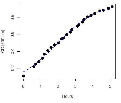
Figure 1. Growth of bacteria over time (optical density at 600 nm UV spectrophotometer), fit by logistic function (dashed line).
Suggested homework
Homework 12: Multiple linear regression.
Quizzes in this chapter
A total of 59 questions among the several subchapters, a mix of true or false and multiple choice question format.