20.9 – Survival analysis
draft
Introduction
As the name suggests, survival analysis is a branch of statistics used to account for death of organisms, or more generally, failure in a system. In general, this kind of analysis models time to event, where event would be death or failure. The basics of the method is defined by the survival function

where  is time,
  is a variable that represents time of death or other end point, and
  is probability of an event occurring later than at time . Two methods are common: the descriptive Kaplan-Meier estimator and the the semi-parametric Cox proportional hazards model.
Excellent resources available, series of articles in volume 89 of British Journal of Cancer: Clark et al (2003a), Bradburn et al (2003a), Bradburn et al (2003b), and Clark et al (2003b).
Hazard function
Defined as the event rate at time t based on survival for time times equal to or greater than t.
Censoring
Censoring is a a missing data problem typical of survival analysis. Distinguish right-censored and left-censored.
Kaplan-Meier plot
Kaplan-Meier (KM) estimator of survival function. Other survival function estimators Fleming-Harrington. The KM estimator,  is
is

where di is the number of events that occurred at time ti, ni is the number of individuals known to have survived or not been censored. Because it’s an estimate, a statistic, need an estimate of the error variance. Several options, the default in R is the Greenwood estimator.

The KM plot, censoring times noted with plus.
R code
Download and install the RcmdrPlugin.survival package.
Example
data(heart, package="survival")
attach(heart)
#Get help with the data set
help("heart", package="survival")
head(heart)
 start stop event        age      year surgery transplant id
1    0   50     1 -17.155373 0.1232033       0          0  1
2    0    6     1   3.835729 0.2546201       0          0  2
3    0    1     0   6.297057 0.2655715       0          0  3
4    1   16     1   6.297057 0.2655715       0          1  3
5    0   36     0  -7.737166 0.4900753       0          0  4
6   36   39     1  -7.737166 0.4900753       0          1  4
Run basic survival analysis. After installing the RcmdrPlugin.survival, from Rcmdr select estimate survival function.
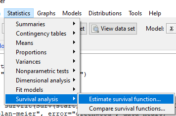
Figure 1. Screenshot of menu call for survival analysis in Rcmdr
Get survival estimator and KM plot (Figure 2)
R output
.Survfit <- survfit(Surv(start, event) ~ 1, conf.type="log", conf.int=0.95,
Rcmdr+ type="kaplan-meier", error="greenwood", data=heart)

 .Survfit
Call: survfit(formula = Surv(start, event) ~ 1, data = heart, error = "greenwood",
conf.type = "log", conf.int = 0.95, type = "kaplan-meier")

n events median 0.95LCL 0.95UCL
172 75 26 17 37

plot(.Survfit, mark.time=TRUE)

quantile(.Survfit, quantiles=c(.25,.5,.75))
$quantile
25 50 75
3 26 67

$lower
25 50 75
1 17 46

$upper
25 50 75
12 37 NA

#by default, Rcmdr removes the object
remove(.Survfit)
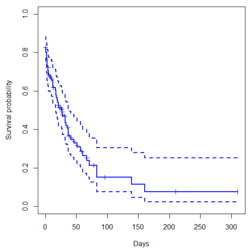
Figure 2. Kaplan-Meier plot of heart data. Dashed lines are upper and lower confidence intervals about the survival function.
Interpreting the plot is straightforward — every time an event occurs, the curve drops.
Note 1: I modified the plot() code with these additions
ylim = c(0,1), ylab="Survival probability", xlab="Days", lwd=2, col="blue"
the data set includes age and whether or not subjects had heart surgery before transplant. Compare.
Variable surgery is recorded 0,1, so need to create a factor
fSurgery <- as.factor(surgery)
Now, to compare
Rcmdr: Statistics → Survival analysis → Compare survival functions…
R output
Rcmdr> survdiff(Surv(start,event) ~ fSurgery, rho=0, data=heart)
Call:
survdiff(formula = Surv(start, event) ~ fSurgery, data = heart,
rho = 0)

              N Observed Expected (O-E)^2/E (O-E)^2/V
fSurgery=No 143       66     58.7     0.902      4.56
fSurgery=Yes 29        9     16.3     3.255      4.56

Chisq= 4.6 on 1 degrees of freedom, p= 0.03
Get the KM estimator and make a KM plot
mySurvfit <- survfit(Surv(start, event) ~ surgery, conf.type="log", conf.int=0.95,
type="kaplan-meier", error="greenwood", data=heart)

plot(mySurvfit, mark.time=TRUE, ylim=c(0,1),lwd=2, col=c("blue","red"), xlab="Number of days", ylab="Survival probability")
legend("topright", legend = paste(c("Surgery - No", "Surgery - Yes")), col = c("blue", "red"), pch = 19, bty = "n")
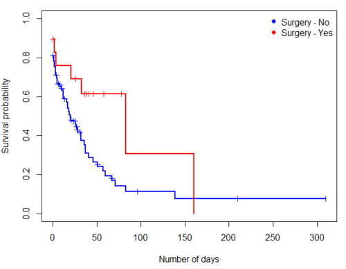
Figure 3. KM plot comparing survival of patients who received surgery (red) and those who did not have the surgery (blue).
The comparison plot can be made in Rcmdr by selecting our Surgery factor in Strata setting (Fig. 4). Recall that strata refers to subgroups of a population.
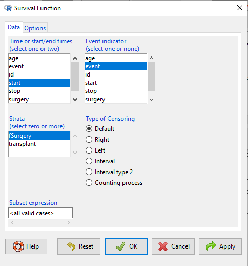
Figure 4. Screenshot of Survival estimator menu in Rcmdr.
Cox proportional hazards model
coxph()
Questions
[pending]
Chapter 20 contents
- Additional topics
- Area under the curve
- Peak detection
- Baseline correction
- Surveys
- Time series
- Dimensional analysis
- Estimating population size
- Diversity indexes
- Survival analysis
- Growth equations and dose response calculations
- Plot a Newick tree
- Phylogenetically independent contrasts
- How to get the distances from a distance tree
- Binary classification
- Meta-analysis
/MD