6.11 – F distribution
Introduction
The F distribution is the probability distribution associated with the F statistic and named in honor of R. A. Fisher. The F distribution is used as the null distribution of the ANOVA test statistic. The F distribution is the ratio of two chi-square distributions, with degrees of freedom v1 and v2 for numerator and denominator, respectively.
Note 1: George W. Snedecor named the F-distribution after Sir Ronald Fisher in honor of his work on variance ratio. Fisher first developed the concept of the variance ratio in the 1920s, calling it the “general z-distribution”.
We can for illustration purposes define the F statistic as a ratio of two variances,

Note 2: We test the ratio of variances to infer the difference between means because a large ratio suggests the variation between groups is much greater than the variation within groups. This comparison, key to Analysis of Variance (ANOVA), allows us to decide if the group means are different beyond random chance.
The F statistic has two sets of degrees of freedom, one for the numerator and one for the denominator. The actual formula for the F distribution is quite complicated and in general we don’t use the F distribution in a way that involves parameter estimation. Rather, it is used in evaluating the statistical significance of the F statistic. Therefore, we produce but a few graphs and a table of critical values to illustrate the distribution.
We call the result of this calculation the F test statistic. We evaluate how often that value or greater of a test statistic will occur by applying the F distribution function. A few graphs to get a sense of what the distribution looks like for varying v1, v2 held to ten degrees of freedom (Fig 1).
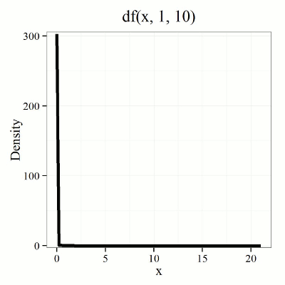
Figure 1. Animated GIF plot of F distribution value for range of degrees of freedom.
By convention in the Null Hypothesis Significance Testing protocol (NHST), we compare the test statistic to a critical value. The critical value is defined as the value of the test statistic that occurs at the Type I error rate, which is typically set to 5%., per our presentations in Chapter 6.7, 6.9, and 6.10. The justification for NHST approach to testing of statistical significance is developed in Chapter 8.
Table of Critical values of the F distribution, one tail (upper)
Degrees of freedom v1 = 1 – 4, v2 = 10
| Fv1, 10 | α = 0.05 | α = 0.025 | α = 0.01 |
| 1 | 4.964 | 6.937 | 10.044 |
| 2 | 4.103 | 5.456 | 7.559 |
| 3 | 3.708 | 4.826 | 6.552 |
| 4 | 3.478 | 4.468 | 5.994 |
For the complete F table see Appendix 20.4
χ2, t and F distributions are related
χ2, t and F distributions are all distributions indexed by their degrees of freedom. With some algebra, these three distributions can be shown to be related to each other. The probabilities tabled in the chi-squared are part of the F-distribution.
Some interesting relationships between the F distribution and other distributions can be shown. By definition we claimed that the F distribution is built on ratio of chi-square distributions, so that should indicate to you the relationship between the two kinds of continuous probability distributions. However, one can also show relationships to other distributions for the F distribution. For example, for the case of v1 = 1 and v2 = any value, then F1,v2 = t2, where t refers to the t distribution.
Questions
- What happens to the shape of the F distribution as df1 is held constant, but df2 degrees of freedom are increased from 1 to 5 to 20 to 100?
- What happens to the shape of the F distribution as df1 degrees of freedom are increased from 1 to 5 to 20 to 100 while df2 is held constant?
Be able to answer these questions using the F table, Appendix 20.4, or using R/Rcmdr
- For probability α = 5%, and numerator degrees of freedom equal to 1, what is the critical value of the F distribution (upper tail) for 5 degree of freedom? For 20 df? For 30 df?
Quiz Chapter 6.11
F distribution
Chapter 6 contents
- Introduction
- Some preliminaries
- Ratios and proportions
- Combinations and permutations
- Types of probability
- Discrete probability distributions
- Continuous distributions
- Normal distribution and the normal deviate (Z)
- Moments
- Chi-square distribution
- t distribution
- F distribution
- References and suggested readings