12.2 – One way ANOVA

Introduction
Three important terms you’ll need for one-way ANOVA
Note on experimental design
ANOVA sources of variation
Mean squares
Worked example with R
Questions
Data set
Chapter 12 contents

Introduction

In ANalysis Of VAriance, or ANOVA for short, we likewise have tools to test the null hypothesis of no difference between between categorical independent variables — often called factors when there’s just a few levels to keep track of — and a single, dependent response variable. But now, the response variable is quantitative, not qualitative like the $\chi^2$ tests.

Analysis of variance, ANOVA, is such an important statistical test in biology that we will take the time to “build it” from scratch. We begin by reminding you of where you’ve been with the material.

We already saw an example of this null hypothesis. When there’s only one factor (but with two or more levels), we call the analysis of means and “one-way ANOVA.” In the independent sample t-test, we tested whether two groups had the same mean. We made the connection between the confidence interval of the difference between the sample means and whether or not it includes zero (i.e., no difference between the means). In ANOVA, we extend this idea to a test of whether two or more groups have the same mean. In fact, if you perform an ANOVA on only two groups, you will get the exact same answer as the independent two-sample t-test, although they use different distributions of critical values (t for the t-test, F for the ANOVA — a nice little fact for you square the t-test statistic, you’ll get the F-test statistic: $t^{2} = F$ ).

Let’s say we have an experiment where we’ve looked at the effect of different three different calorie levels on weight change in middle-aged men.

I’ve created a simulated dataset which we will use in our ANOVA discussions. The data set is available at the end of this page (scroll down or click here).

We might graph the mean weight changes ( $\pm$ SEM); Below are two possible outcomes of our experiment (Fig. 1).

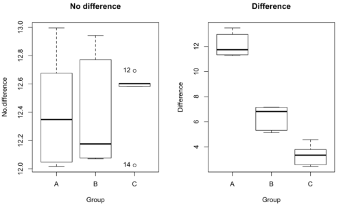
Figure 1. Hypothetical results, box plots.

Figure 1. Hypothetical results of an experiment, box plots. Left, no difference among groups; Right, large differences among groups.

As statisticians and scientists, we would first calculate an overall or grand mean for the entire sample of observations; we know this as the sample mean whose symbol is $\bar{X}$ . But this overall mean is made up of the average of the sample means. If the null hypothesis is true, then the all of the sample means all estimate the overall mean. Put another way, being a member of a treatment group doesn’t matter, i.e., there is no systematic effect, all differences among subjects are due to random chance.

$\begin{align*} H_{0} : \bar{X} = \bar{X}_{A} = \bar{X}_{B} = \bar{X}_{C} \end{align*}$

The hypotheses among are three groups or treatment levels then are:

$\begin{align*} H_{0} : \bar{X}_{A} = \bar{X}_{B} = \bar{X}_{C}&& \end{align*}$

Null that there are no differences among the group means. And the alternative hypotheses include any (or all) of the following possibilities

$\begin{align*} H_{0} : \bar{X}_{A} \ne \bar{X}_{B} = \bar{X}_{C} \end{align*}$

or maybe

$\begin{align*} H_{0} : \bar{X}_{A} = \bar{X}_{B} \ne \bar{X}_{C} \end{align*}$

or… have we covered all possible alternate outcomes among three groups?

In either case, we could use one-way ANOVA to test for “statistically significant differences.”

Three important terms you’ll need for one-way ANOVA

FACTOR: We have one factor of interest. For example, a factor of interest might be

Diet fed to hypertensive subjects (men and women)
Distribution of coral reef sea cucumber species in archipelagos
Antibiotic drug therapy for adolescents with Acne vulgaris (click see Webster 2002 for review).

Note: Character vs factor. In R programming, while it is true that a treatment variable can be a character vector like Gender*, such vectors are handled by R as string. In contrast, by claiming Gender as a factor, R handles the variable as a nominal data type. Hence, ANOVA and other GLM functions expect any treatment variable to be declared as a factor:

Gender <- c("Gender non-conforming", "Men", "Non-binary", "Transgender", "Women", "Declined"); Gender
[1] "Gender non-conforming" "Men" "Non-binary" "Transgender" 
[5] "Women" "Declined"

# it’s a string vector, not a factor

is.factor(Gender)
[1] FALSE

Change string vector to a factor.

Gender <- as.factor(Gender); is.factor(Gender) [1] TRUE

* For discussions of ethics of language inclusivity and whether or not such information should be gathered, see Henrickson et al 2020.

LEVELS: We can have multiple levels (2 or more) within the single factor. Some examples of levels for the Factors listed:

Three diets (DASH), diet rich in fruits & vegetables, control diet)
Five archipelagos (Hawaiian Islands, Line Islands, Marshal Islands, Bonin Islands, and Ryukyu Islands)
Five antibiotics (ciprofloxacin, cotrimoxazole, erythromycin, doxycycline, minocycline).

RESPONSE: There is one outcome or measurement variable. This variable must be quantitative (i.e., on the ratio or interval scale). Continuing our examples then

Reduction in systolic pressure
Numbers of individual sea cucumbers in a plot
number of microcomedo†.

†A comedo is a clogged pore in the skin; a microcomedo refers to the small plug. Yes, I had to look that up, too.

The response variable can be just about anything we can measure, but because ANOVA is a parametric test, the response variable must be normally distributed!

Note on experimental design

As we discuss ANOVA, keep in mind we are talking about analyzing results from an experiment. Understanding statistics, and in particular ANOVA, informs how to plan an experiment. The basic experimental design is called a completely randomized experimental design, or CDR, where treatments are assigned to experimental units at random.

In this experimental design, subjects (experimental units) must be randomly assigned to each of these levels of the factor. That is, each individual should have had the same probability of being found in any one of the levels of the factor. The design is complete because randomization is conducted for all levels, all factors.

Thinking about how you would describe an experiment with three levels of some treatment, we would have

Table 1. Summary statistics of three levels for some ratio scale response variable.

Level 1

$\bar_{X}_{1}$

sample mean₁

$s_{1}$

sample standard deviation₁

Level 2

$\bar_{X}_{2}$

sample mean₂

$s_{2}$

sample standard deviation₂

Level 3

$\bar_{X}_{3}$

sample mean₃

$s_{3}$

sample standard deviation₃

Note: this table is the basis for creating the box plots in Figure 1.

ANOVA sources of variation

ANOVA works by partitioning total variability about the means (the grand mean, the group means). We will discuss the multiple samples and how the ANOVA works in terms of the sources of variation. There are two “sources” of variation that can occur:

Within Group Variation
Among Groups Variation

So let’s look first at the variability within groups, also called the Within Group Variation.

Consider and experiment to see if DASH diet reduces systolic blood pressure in USA middle-aged men and women with hypertension (Moore et al 2001). After eight weeks we have

We get the corrected sum of squares, SS, for within group

$\begin{align*} within-groups \ SS = \sum_{i=1}^{k}\left [ \sum_{j=1}^{n_{i}}\left ( X_{ij}-\bar{X}_{i} \right )^2 \right ] \end{align*}$

and the degrees of freedom, DF, for within groups

$\begin{align*} within-groups \ DF = \sum_{i=1}^{k}\left ( n_{i}-1 \right ) = N - k \end{align*}$

where i is the identity of the groups, $X_{ij}$ is the individual observations within group i, $\bar{X}_{i}$ is the group i mean, n_i is the sample size within each group, N is the total sample size of all subjects for all groups, and k is the number of groups.

Importantly, this value is also referred to as “error sums of squares” in ANOVA. It’s importance is as follows — In our example, the within group variability would be zero if and only if all subjects within the same diet lost exactly the same amount of weight. This is hardly ever the case of course in a real experiment. Because there are almost always some other unknown factors or measurement error that affect the response variable, there will be some unknown variation among individuals who received the same treatment (within the same group). Thus, the error variance will generally be larger than zero.

The first point to consider: your ANOVA will never result in statistical differences among the groups if the error variance is greater than the second type of variability, the variability between groups.

The second type of variability in ANOVA is that due to the groups or treatments. Individuals given a calorie-restricted diet will loose some weight; individuals allowed to eat a calorie-rich diet likely will gain weight, therefore there will be variability (a difference) due to the treatment. So we can calculate the variability among groups. We get the corrected sum of squares for among groups

$\begin{align*} among-groups \ SS = \sum_{i=1}^{k}n_{i}\left ( X_{i}-\bar{X}\right )^2 \end{align*}$

and the degrees of freedom for among groups

$\begin{align*} among-groups \ DF = k - 1 \end{align*}$

where i is the identity of the groups, $\bar{X}$ is the grand mean as defined in Measures of Central Tendency (Chapter 3.1), $\bar{X}_{i}$ is the group i mean, n_i is the sample size within each group, N is the total sample size of all subjects for all groups, and k is the number of groups.

The sums of squares here is simply subtracting the mean of each population from the overall mean.

If the Factor is not important in explaining the variation among individuals then all the population means will be similar and the sums of squares among populations would be small.
If the Factor is important in explaining some of the variation among the individuals then all the population means will NOT be the same and the sums of squares among populations would be large.

Finally, we can identify the total variation in the entire experiment. We have the total sum of squares.

$\begin{align*} Total \ SS = among-groups \ SS + within-groups \ SS \end{align*}$

Thus, the insight of ANOVA is that variation in the dataset may be attributed to a portion explained by differences among the groups and differences among individual observations within each group. The inference comes from recognizing that if the among group effect is greater than the within group effect, then there will be a difference due to the treatment levels.

Mean squares

To decide whether the variation associated with the among group differences are greater than the within group variation, we calculate ratios of the sums of squares. These are called Mean Squares or MS for short. The ratio of the Mean Squares is called F, the test statistic for ANOVA.

For the one-way ANOVA we will have two Mean Squares and one F, tested with degrees of freedom for both the numerator $MS_{groups}$ , and denominator $MS_{error}$ ).

The Mean Square for (among) groups is

$\begin{align*} MS_{group} = \frac{among-groups \ SS}{among-groups \ DF} \end{align*}$

The Mean Square for error is

$\begin{align*} MS_{error} = \frac{within-groups \ SS}{within-groups \ DF} \end{align*}$

And finally, the value for F, the test statistic for ANOVA, is

$\begin{align*} F = \frac{MS_{group}}{MS_{error}} \end{align*}$

Worked example with R

A factor with three levels, A, B, and C

group <- c("A", "A", "A", "B", "B", "B", "C", "C", "C")

and their responses, simulated

response <- c(10.8, 11.8, 12.8, 6.5, 7, 8, 3.8, 2.8, 3)

We create a data frame

all <- data.frame(group, response)

Of course, you could place the data into a worksheet and then import the worksheet into R. Regardless, we now have our dataset.

Now, call the ANOVA function, aov, and assign the results to an object (e.g., Model.1)

Model.1 <- aov(response ~ group, data=all)

Now, visualize the ANOVA table

summary(Model.1)

and the output from R, the ANOVA table, is shown below

Rcmdr: Statistics → Means → One-way ANOVA… see figures 2 and 3 below

Table 2. Output from aov() command, the ANOVA table, for the “Difference” outcome variable.

           Df   Sum Sq    Mean Sq   F value       Pr(>F) 
group       2   111.16      55.58     89.49    0.0000341 ***
Residuals   6     3.73       0.62
---
Signif. codes: 0 '***' 0.001 '**' 0.01 '*' 0.05 '.' 0.1 ' ' 1

Let’s take the ANOVA table one row at a time

The first row has subject headers defining the columns.
The second row of the table “groups” contains statistics due to group, and provides the comparisons among groups.
The third row, “Residuals” is the error, or the differences within groups.

Moving across the columns, then, for each row, we have in turn,

the degrees of freedom (there were 3 groups, therefore 2 DF for group),
the Sums of Squares, the Mean Squares,
the value of F, and finally,
the P-value.

R provides a helpful guide on the last line of the ANOVA summary table, the “Signif[icance] codes,” which highlights the magnitude of the P-value.

What to report? ANOVA problems can be much more complicated than the simple one-way ANOVA introduced here. For complex ANOVA problems, report the ANOVA table itself! But for the one-way ANOVA it would be sufficient to report the test statistic, the degrees of freedom, and the p-value, as we have in previous chapters (e.g., t-test, chi-square, etc.). Thus, we would report:

F = 89.49, df = 2 and 6, p = 0.0000341

where F = 89.49 is the test statistic, df = 2 (degrees of freedom for the among group mean square) and 6 (degrees of freedom for the within group mean square), and p = 0.0000341 is the p-value.

In Rcmdr, the appropriate command for the one-way ANOVA is simply

Rcmdr: Statistics → Means

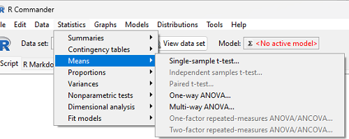
Screenshot Rcmdr select one-way ANOVA

Figure 2. Screenshot Rcmdr select one-way ANOVA

which brings up a simple dialog. R Commander anticipates factor (Groups) and Response variable. Optional, choose Pairwise comparisons of means for post-hoc test (Tukey’s) and, if you do not want to assume equal variances (see Chapter 13), select Welch F-test.

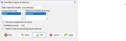
Screenshot Rcmdr select one-way ANOVA options

Figure 3. Screenshot Rcmdr select one-way ANOVA options.

Questions

1. Review the example ANOVA Table and confirm the following

How many levels of the treatment were there?
How many sampling units were there?
Confirm the calculation of $MS_{group}$ and $MS_{error}$ using the formulas contained in the text.
Confirm the calculation of F using the formula contained in the text.
The degrees of freedom for the F statistic in this example were 2 and 6 (F_2,6). Assuming a two-tailed test with Type I error rate of 5%, What is the critical value of the F distribution (see Appendix 20.4)

2. Repeat the one-way ANOVA using the simulated data, but this time, calculate the ANOVA problem for the “No.difference” response variable.

3. Leaf lengths from three strains of Arabidopsis thaliana plants grown in common garden are shown in Fig. 2. Data are provided for you in the following R script.

arabid <- c("wt","wt","wt","AS1","AS1","AS1","AS2","AS2","AS2")
leaf <- c(4.909,5.736,5.108,6.956,5.809,6.888,4.768,4.209,4.065)
leaves <- data.frame(arabid,leaf)

Write out a null and alternative hypotheses
Conduct a test of the null hypothesis by one-way ANOVA
Report the value of the test statistic, the degrees of freedom, and the P-value
Do you accept or reject the null hypothesis? Explain your choice.

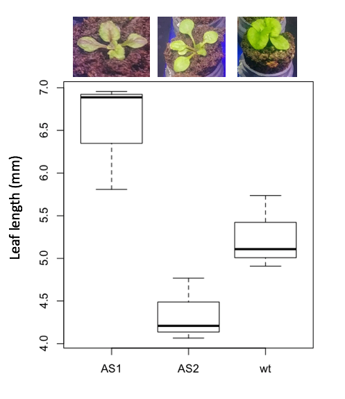
Box plot of length of leaves from three strains of Arabidopsis thaliana

Figure 4. Box plot of lengths of leaves of a 10-day old plant from on of three strains of Arabidopsis thaliana.

4. Return to your answer to question 7 from Chapter 12.1 and review your answer and modify as appropriate to correct your language to that presented here about factors and levels.

5. Conduct the one-way ANOVA test on the Comet assay data presented question 7 from Chapter 12.1. Data are copied for your convenience to end of this page. Obtain the ANOVA table and report the value of the test statistics, degrees of freedom, and p-value.
a. Based on the ANOVA results, do you accept or reject the null hypothesis? Explain your choice.

Data used in this page

Difference, no difference

Table 12.2 Difference or No Difference

Group	No.difference	Difference
A	12.04822	11.336161
A	12.67584	13.476142
A	12.99568	12.96121
A	12.01745	11.746712
A	12.34854	11.275492
B	12.17643	7.167262
B	12.77201	5.136788
B	12.07137	6.820242
B	12.94258	5.318743
B	12.0767	7.153992
C	12.58212	3.344218
C	12.69263	3.792337
C	12.60226	2.444438
C	12.02534	2.576014
C	12.6042	4.575672

Simulated data

Comet assay, antioxidant properties of tea

Data presented in Chapter 12.1