9.1 – Chi-square test: Goodness of fit
Introduction
We ask about the “fit” of our data against predictions from theory, or from rules that set our expectations for the frequency of particular outcomes drawn from outside the experiment. Three examples to illustrate goodness of fit, GOF,  , A, B, and C follow.
A. For example, for a toss of a coin, we expect heads to show up 50% of the time. Out of 120 tosses of a fair coin, we expect 60 heads, 60 tails. Thus, our null hypothesis would be that heads would appear 50% of the time. If we observe 70 heads in an experiment of coin tossing, is this a significantly large enough discrepancy to reject the null hypothesis?
B. For example, simple Mendelian genetics makes predictions about how often we should expect particular combinations of phenotypes in the offspring when the phenotype is controlled by one gene, with 2 alleles and a particular kind of dominance.
For example, for a one locus, two allele system (one gene, two different copies like R and r) with complete dominance, we expect the phenotypic (what you see) ratio will be 3:1 (or  round,
  wrinkle). Our null hypothesis would be that pea shape will obey Mendelian ratios (3:1). Mendel’s round versus wrinkled peas (RR or Rr genotypes give round peas, only rr results in wrinkled peas).
Thus, out of 100 individuals, we would expect 75 round and 25 wrinkled. If we observe 84 round and 16 wrinkled, is this a significantly large enough discrepancy to reject the null hypothesis?
C. For yet another example, in population genetics, we can ask whether genotypic frequencies (how often a particular copy of a gene appears in a population) follow expectations from Hardy-Weinberg model (the null hypothesis would be that they do).
This is a common test one might perform on DNA or protein data from electrophoresis analysis. Hardy-Weinberg is a simple quadratic expansion:
If p = allele frequency of the first copy, and q = allele frequency of the second copy, then p + q = 1,
Given the allele frequencies, then genotypic frequencies would be given by 1 = p2 + 2pq + q2.
Deviations from Hardy-Weinberg expectations may indicate a number of possible causes of allele change (including natural selection, genetic drift, migration).
Thus, if a gene has two alleles,  and
and  , with the frequency for ,
  and for ,
  (equivalently q = 1 – p) in the population, then we would expect 36
  , 16
, 16  , and 48
  individuals. (Nothing changes if we represent the alleles as A and a, or some other system, eg, dominance/recessive.)
Question. If we observe the following genotypes: 45 individuals, 34 individuals, and 21 individuals, is this a significantly large enough discrepancy to reject the null hypothesis?
Table 1. Summary of our Hardy Weinberg question
| Genotype | Expected | Observed | O – E |
| aa | 70 | 45 | -25 |
| aa’ | 27 | 34 | 7 |
| a’a’ | 3 | 21 | 18 |
| sum | 100 | 100 | 0 |
Recall from your genetics class that we can get the allele frequency values from the genotype values, eg,

We call these chi-square tests, tests of goodness of fit. Because we have some theory, in this case Mendelian genetics, or guidance, separate from the study itself, to help us calculate expected values in a chi-square test.
Note 1: The idea of fit in statistics can be reframed as how well does a particular statistical model fit the observed data. A good fit can be summarized by accounting for the differences between the observed values and the comparable values predicted by the model.
Note also for our coin toss example, goodness of fit isn’t exactly proper terminology — afterall the test is equal probability of the two outcomes, not whether we have match between an observed distribution and an expected distribution (true statement if we add “follows a binomial distribution”).
 goodness of fit
For k groups, the equation for the chi-square test may be written as

where fi is the frequency (count) observed (in class i) and fi<hat> is the frequency (count) expected if the null hypothesis is true, sum over all k groups. Alternatively, here is a format for the same equation that may be more familiar to you… ?

where Oi is the frequency (count) observed (in class i) and Ei is the frequency (count) expected if the null hypothesis is true.
The degrees of freedom, df, for the GOF are simply the number of categories minus one, k – 1.
Explaining GOF
Why am I using the phrase “goodness of fit?” This concept has broad use in statistics, but in general it applies when we ask how well a statistical model fits the observed data.
At least for the chi-square test it is simple to see how the test statistic increases from zero as the agreement between observed data and expected data depart, where zero would be the case in which all observed values for the categories exactly match the expected values.
The goodness of fit test is designed to evaluate whether or not your data agree with a theoretical expectation (there are additional ways to think about this test, but this is a good place to start). Let’s take our time here and work with an example. The other type of chi-square problem or experiment is one for the many types of experiments in which the response variable is discrete, just like in the GOF case, but we have no theory to guide us in deciding how to obtain the expected values. We can use the data themselves to calculate expected values, and we say that the test is “contingent” upon the data, hence these types of chi-square tests are called contingency tables.
You may be a little concerned at this point that there are two kinds of chi-square problems, goodness of fit and contingency tables. We’ll deal directly with contingency tables in the next section, but for now, I wanted to make a few generalizations.
- Both goodness of fit and contingency tables use the same chi-square equation and analysis. They differ in how the degrees of freedom are calculated.
- Thus, what all chi-square problems have in common, whether goodness of fit or contingency table problems
- You must identify what types of data are appropriate for this statistical procedure? Categorical (nominal data type).
- As always, a clear description of the hypotheses being examined.
For goodness of fit chi-square test, the most important type of hypothesis is called a Null Hypothesis: In most cases the Null Hypothesis (HO) is “no difference” “no effect”…. If HO is concluded to be false (rejected), then an alternative hypothesis (HA) will be assumed to be true. Both are specified before tests are conducted. All possible outcomes are accounted for by the two hypotheses.
From above, we have
- A. HO: Fifty out of 100 tosses will result in heads.
- HA: Heads will not appear 50 times out of 100.
- B. HO: Pea shape will equal Mendelian ratios (3:1).
- HA: Pea shape will not equal Mendelian ratios (3:1).
- C. HO: Genotypic frequencies will equal Hardy-Weinberg expectations.
- HA: Genotypic frequencies will not equal Hardy-Weinberg expectations
Assumptions: In order to use the chi-square, there must be two or more categories. Each observation must be in one and only one category. If some of the observations are truly halfway between two categories then you must make a new category (eg, low, middle, high) or use another statistical procedure. Additionally, your expected values are required to be integers, not ratio. The number of observed and the number of expected must sum to the same total.
The chi-square test is a good example of such tests, and we will encounter other examples too. Another common goodness of fit is the coefficient of determination, which will be introduced in linear regression sections (see Chapter 17.7 – Regression model fit). Still other examples are the likelihood ratio test (LRT), Akaike Information Criterion (AIC), and Bayesian Information Criterion (BIC), which are all used to assess fit of models to data. (See Graffelman and Weir [2018] for how to use AIC in the context of testing for Hardy Weinberg equilibrium.)
The likelihood ratio test is used to compare the goodness of fit of two hierarchically nested models to determine if a more complex model provides a significantly better fit to the data. It does this by forming a ratio of the likelihood of the data under the two models (the simpler “null” model and the more complex “alternative” model). A small ratio suggests the simpler model is a poor fit, while a value close to one indicates the added complexity is not statistically significant. AIC (and BIC) is a measure of relative fit — it balances goodness of fit and model complexity: A lower AIC suggests a better model by finding the optimal trade-off between fitting the data well and keeping the model simple. A model that is too complex will have a higher AIC than a simpler model with a nearly as good fit.
We use LRT, AIC and BIC when we talk about selecting best regression models (see Chapter 17.7 – Regression model fit). However, as we discuss the concept of comparing models, we need to distinguish between the concept of model choice — methods used to select a best model from competing options and estimating the “goodness of fit” of a single model.
How well does data fit the prediction?
Frequentist approach interprets the test as, how well does the data fit the null hypothesis,  ? When you compare data against a theoretical distribution (eg, Mendel’s hypothesis predicts the distribution of progeny phenotypes for a particular genetic system), you test the fit of the data against the model’s predictions (expectations). Recall that the Bayesian approach asks how well does the model fit the data?
Table 2. A. 120 tosses of a coin, we count heads 70/120 tosses.
| Expected | Observed | |
| Heads | 60 | 70 |
| Tails | 60 | 50 |
| n | 120 | 120 |

Table 3. B. A possible Mendelian system of inheritance for a one gene, two allele system with complete dominance, observe the phenotypes.
| Expected | Observed | |
| Round | 75 | 84 |
| Wrinkled | 25 | 16 |
| n | 100 | 100 |

Table 4. C. A possible Mendelian system of inheritance for a one gene, two allele system with complete dominance, observe the phenotypes.
| Expected | Observed | |
| p2 | 70 | 45 |
| 2pq | 27 | 34 |
| q2 | 3 | 21 |
| n | 100 | 100 |

For completeness, instead of a goodness of fit test we can treat this problem as a test of independence, a contingency table problem. We’ll discuss contingency tables more in the next section, but or now, we can rearrange our table of observed genotypes for problem C, as a 2X2 table
Table 5. Problem C reported in 2X2 table format.
| Maternal a’ | Paternal a’ | |
| Maternal a | 45 | 17 |
| Paternal a | 17 | 21 |
The contingency table is calculated the same way as the GOF version, but the degrees of freedom are calculated differently: df = number of rows – 1 multiplied by the number of columns – 1.

Thus, for a 2X2 table the df are always equal to 1.
Note that the chi-square value itself says nothing about how any discrepancy between expectation and observed genotype frequencies come about. Therefore, one can rearrange the equation to make clear where deviance from equilibrium, D, occur for the heterozygote (het). We have

where D2 is equal to

φ coefficient
The chi-square test statistic and its inference tells you about the significance of the association, but not the strength or effect size of the association. Not surprisingly, Pearson (1904) came up with a statistic to quantify the strength of association between two binary variables, now called the φ (phi) coefficient. Like the Pearson product moment correlation, the φ (phi) coefficient takes values from -1 to +1.
Note 2: Pearson termed this statistic the mean square contingency coefficient. Yule (1912) termed it the phi coefficient. The correlation between two binary variables is also called the Mathews Correlation Coefficient or MCC (Mathews 1975), which is a common classification tool in machine learning.
The formula for the absolute value of φ coefficient is

Thus, for A, B, and C examples, φ coefficient was 0.167, 0.190, and 0.771. Thus, only weak associations in examples A and B, but strong association in C. We’ll provide a formula to directly calculate φ coefficient from the cells of the table in 9.2 – Chi-square contingency tables.
Carry out the test and interpret results
What was just calculated? The chi-square, , test statistic.
Just like t-tests, we now want to compare our test statistic against a critical value — calculate degrees of freedom (df = k – 1, k equals the numbers of categories), and set a rejection level, Type I error rate. We typically set the Type I error rate at 5%. A table of critical values for the chi-square test is available in Appendix Table Chi-square critical values.
Obtaining Probability Values for the goodness-of-fit test of the null hypothesis:
As you can see from the equation of the chi-square, a perfect fit between the observed and the expected would be a chi-square of zero. Thus, asking about statistical significance in the chi-square test is the same as asking if your test statistic is significantly greater than zero.
The chi-square distribution is used and the critical values depend on the degrees of freedom. Fortunately for and other statistical procedures we have Tables that will tell us what the probability is of obtaining our results when the null hypothesis is true (in the population).
Here is a portion of the chi-square critical values for probability that your chi-square test statistic is less than the critical value (Fig 1).
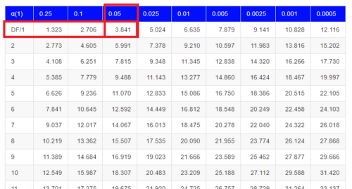
Figure 1. A portion of critical values of the chi-square at alpha 5% for degrees of freedom between 1 and 10. A more inclusive table is provided in the Appendix, Table of Chi-square critical values.
For the first example (A), we have df = 2 – 1 = 1 and we look up the critical value corresponding to the probability in which Type I = 5% are likely to be smaller iff (“if and only if”) the null hypothesis is true. That value is 3.841; our test statistic was 3.330, and therefore smaller than the critical value: so we do not reject the null hypothesis.
Interpolating p-values
How likely is our test statistic value of 3.333 and the null hypothesis was true? (Remember, “true” in this case is a shorthand for our data was sampled from a population in which the HW expectations hold). When I check the table of critical values of the chi-square test for the “exact” p-value, I find that our test statistic value falls between a p-value 0.10 and 0.05 (represented in the table below). We can interpolate
Note 3: Interpolation refers to any method used to estimate a new value from a set of known values. Thus, interpolated values fall between known values. Extrapolation on the other hand refers to methods to estimate new values by extending from a known sequence of values.
Table 6. Interpolated p-value for critical value not reported in chi-square table.
| statistic | p-value |
| 3.841 | 0.05 |
| 3.333 | x |
| 2.706 | 0.10 |
If we assume the change in probability between 2.706 and 3.841 for the chi-square distribution is linear (it’s not, but it’s close), then we can do so simple interpolation.
We set up what we know on the right hand side equal to what we don’t know on the left hand side of the equation,

and solve for x. Then, x is equal to 0.0724
R function pchisq() gives a value of p = 0.0679. Close, but not the same. Of course, you should go with the result from R over interpolation; we mention how to get the approximate p-value by interpolation for completeness, and, in some rare instances, you might need to make the calculation. Interpolating is also a skill used to provide estimates where the researcher needs to estimate (impute) a missing value.
Interpreting p-values
This is a pretty important topic, so much so that we devote an entire section to this very problem — see 8.2 – The controversy over proper hypothesis testing. If you skipped the chapter, but find yourself unsure how to interpret the p-value, then please go back to Ch 8.2. OK, that commercial message, what does it mean to “reject the chi-square null hypothesis?” These types of tests are called goodness of fit in the following sense — if your data agree with the theoretical distribution, then the difference between observed and expected should be very close to zero. If it is exactly zero, then you have a perfect fit. In our coin toss case, if we say that the ratio of heads:tails do not differ significantly from the 50:50 expectation, then we accept the null hypothesis.
You should try the other examples yourself! A hint, the degrees of freedom are one (1) for example B and two (2) for example C.
R code
Printed tables of the critical values from the chi-square distribution, or for any statistical test for that matter are fine, but with your statistical package R and Rcmdr, you have access to the critical value and the p-value of your test statistic simply by asking. Here’s how to get both.
First, let’s get the critical value.
Rcmdr: Distributions → Continuous distributions → Chi-squared distribution → Chi-squared quantiles (Fig 2).
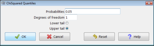
Figure 2. R Commander menu for Chi-squared quantiles.
I entered “0.05” for the probability because that’s my Type I error rate α. Enter “1” for Degrees of freedom, then click “upper tail” because we are interested in obtaining the critical value for α. Here’s R’s response when I clicked “OK.”
qchisq(c(0.05), df=1, lower.tail=FALSE)
[1] 3.841459
Next, let’s get the exact P-value of our test statistic. We had three from three different tests:  for the coin-tossing example,
  for the pea example, and
  for the Hardy-Weinberg example.
Rcmdr: Distributions → Continuous distributions → Chi-squared distribution → Chi-squared probabilities… (Fig 3).
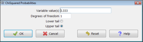
Figure 3. R Commander menu for Chi-squared probabilities.
I entered “3.333” because that is one of the test statistics I want to calculate for probability and “1” for Degrees of freedom because I had k – 1 = 1 df for this problem. Here’s R’s response when I clicked “OK.”
pchisq(c(3.333), df=1, lower.tail=FALSE)
[1] 0.06790291
I repeated this exercise for I got  ; for I got
  .
.
Nice, right? Saves you from having to interpolate probability values from the chi-square table.
3. How to get the goodness of fit in Rcmdr.
R provides the goodness of fit (the command is chisq.text()), but Rcmdr thus far does not provide a menu option to link to the function. Instead, R Commander provides a menu for contingency tables, which also is a chi-square test, but is used where no theory is available to calculate the expected values (see Chapter 9.2). Thus, for the goodness of fit chi-square, we will need to bypass Rcmdr in favor of the script window. Honestly, other options are as quick or quicker: calculate by hand, use a different software (eg, Microsoft Excel), or many online sites provide JavaScript tools.
So how to get the goodness of fit chi-square while in R? Here’s one way. At the command line, type
chisq.test (c(O1, O2, ... On), p = c(E1, E2, ... En))
where O1, O2, … On are observed counts for category 1, category 2, up to category n, and E1, E2, … En are the expected proportions for each category. For example, consider our Heads/Tails example above (problem A).
In R, we write and submit
chisq.test(c(70,30),p=c(1/2,1/2))
R returns
Chi-squared test for given probabilities.
data: c(70, 30)
X-squared = 16, df = 1, p-value = 0.00006334
Easy enough. But not much detail — details are available with some additions to the R script. I’ll just link you to a nice website that shows how to add to the output so that it looks like the one below.
mike.chi <- chisq.test(c(70,30),p=c(1/2,1/2))
Let’s explore one at time the contents of the results from the chi square function.
names(mike.chi)   #The names function
[1] "statistic" "parameter" "p.value" "method" "data.name" "observed"
[7] "expected" "residuals" "stdres"
Now, call each name in turn.
mike.chi$residuals
[1] 2.828427 -2.828427
mike.chi$obs
[1] 70 30
mike.chi$exp
[1] 50 50
Note 4: “residuals” here simply refers to the difference between observed and expected values. Residuals are an important concept in regression, see Ch17.5
And finally, let’s get the summary output of our statistical test.
mike.chi
Chi-squared test for given probabilities.
data: c(70, 30)
X-squared = 16, df = 1, p-value = 6.334e-05
GOF and spreadsheet apps
Easy enough with R, but it may even easier with other tools. I’ll show you how to do this with spreadsheet apps and with and online at graphpad.com.
Let’s take the pea example above. We had 16 wrinkled, 84 round. We expect 25% wrinkled, 75% round.
Now, with R, we would enter
chisq.test(c(16,80),p=c(1/4,3/4))
and the R output
Chi-squared test for given probabilities
data: c(16, 80)
X-squared = 3.5556, df = 1, p-value = 0.05935
Microsoft Excel and the other spreadsheet programs (Apple Numbers, Google Sheets, LibreOffice Calc) can calculate the goodness of fit directly; they return a P-value only. If the observed data are in cells A1 and A2, and the expected values are in B1 and B2, then use the procedure =CHITEST(A1:A2,B1:B2).
Table 7. A spreadsheet with formula visible.
| A | B | C | D | |
| 1 | 80 | 75 | ||
| 2 | 16 | 25 | =CHITEST(A1:A2,B1:B2) |
The P-value (but not the Chi-square test statistic) is returned. Here’s the output from Calc.
Table 8. Spreadsheet example from Table 7 with calculated P-value.
| A | B | C | D | |
| 1 | 80 | 75 | ||
| 2 | 16 | 25 | 0.058714340077662 |
You can get the critical value from MS Excel (=CHIINV(alpha, df), returns the critical value), and the exact probability for the test statistic =CHIDIST(x,df), where x is your test statistic. Putting it all together, a general spreadsheet template for goodness of fit calculations calculations of test statistic and p-value might look like
Table 9. Spreadsheet template with formula to calculate chi-square goodness of fit on two groups.
| A | B | C | D | E | |
| 1 | f1 | 0.75 | |||
| 2 | f2 | 0.25 | |||
| 3 | N | =SUM(A5,A6) |
|||
| 4 | Obs | Exp | Chi.value | Chi.sqr | |
| 5 | 80 | =B1* |
=((A5-B5)^2)/B5 |
=SUM(C5,C6) |
|
| 6 | 16 | =B2* |
=((A6-B6)^2)/B6 |
=CHIDIST(D5, COUNT(A5:A6-1) |
|
| 7 | |||||
| 8 |
 3
3Microsoft Excel can be improved by writing macros, or by including available add-in programs, such as the free PopTools, which is available for Microsoft Windows 32-bit operating systems only.
Another option is to take advantage of the internet — again, many folks have provided java or JavaScript-based statistical routines for educational purposes. Here’s an easy one to use www.graphpad.com.
In most cases, I find the chi-square goodness-of-fit is so simple to calculate by hand that the computer is redundant.
Questions
1. A variety of p-values were reported on this page with no attempt to reflect significant figures or numbers of digits (see Chapter 8.2). Provide proper significant figures and numbers of digits as if these p-values were reported in a science journal.
- 0.0724
- 0.0679
- 0.03766692
- 0.004955794
- 0.00006334
- 6.334e-05
- 0.05935
- 0.058714340077662
2. For a mini bag of M&M candies, you count 4 blue, 2 brown, 1 green, 3 orange, 4 red, and 2 yellow candies.
- What are the expected values for each color?
- Calculate using your favorite spreadsheet app (eg, Numbers, Excel, Google Sheets, LibreOffice Calc)
- Calculate using R (note R will reply with a warning message that the “Chi-squared approximation may be incorrect”; see 9.2 Yates continuity correction)
- Calculate using Quickcalcs at graphpad.com
- Construct a table and compare p-values obtained from the different applications
3. CYP1A2 enzyme involved with metabolism of caffeine. Folks with C at SNP rs762551 have higher enzyme activity than folks with A. Populations differ for the frequency of C. Using R or your favorite spreadsheet application, compare the following populations against global frequency of C is 33% (frequency of A is 67%).
- 286 persons from Northern Sweden: f(C) = 26%, f(A) = 73%
- 4532 Native Hawaiian persons: f(C) = 22%, f(A) = 78%
- 1260 Native American persons: f(C) = 30%, f(A) = 70%
- 8316 Native American persons: f(C) = 36%, f(A) = 64%
- Construct a table and compare p-values obtained for the four populations.
Quiz Chapter 9.1
Chi-square test: Goodness of fit