1.1 – A quick look at R and R Commander
A first look at R
.
R is a programming language for statistical computing (Venables et al 2009). R is an interpreted language — when you run (execute) an R program — the R interpreter intercepts and runs the code immediately through its command-line interface, one line at time. Python is another popular interpreted language common in data science. Interpreted languages are in contrast to compiled languages, like C++ and Rust, where program code is sent to a compiler to a machine language application.
The following steps user through use of R and R Commander, from installation to writing and running commands. Mike’s Workbook for Biostatistics has a ten-part tutorial, A quick look at R and R Commander, which I recommend.
Note: Getting started? By all means rely on Mike’s Biostatistics Book and blogs or other online tutorials to point you in the right direction. You’ll also find many free and online books that may provide the right voice to get you working with R. However, the best way to learn is to go to the source. The R team has provided extensive documentation, all included as part of your installation of R. In R, run the command RShowDoc("doc name"). replace doc name with the name of the R manual or R user guide. For example, the Venables publication is accessed as RShowDoc("R-intro"). Similarly, the manual for installation is RShowDoc("R-admin") and the manual for R data import/export is RShowDoc("R-data").
Install R
.
Full installation instructions are available at Install R and for the R Commander package, at Install R Commander. Here, we provide a brief overview of the installation process.
Note: The instructions at Mike’s Biostatistics Book assume use of R on a personal computer running updated Microsoft Windows or Apple macOS operating systems. For Linux instructions, e.g., Ubuntu distro, see How to install R on Ubuntu 22.04. For Chromebook users, if you can install a Linux subsystem, then you can also install and run R although it’s not a trivial installation. For instructions to install R see Levi’s excellent writeup at levente.littvay.hu/chromebook/. (This works best with Intel-based CPUs — see my initial attempts with an inexpensive Chromebook at Install R).
Another option is to run R in the cloud via service like Google’s Colab or CoCalc hosted by SageMath. Both support Jupyter Notebooks, a “web-based interactive computational environment.” Neither cloud-based service supports use of R Commander (because R Commander interacts with your local hardware). Colab is the route I’d choose if I don’t have access to a local installation of R.
Download a copy of the R installation file appropriate for your computer from one of the Comprehensive R Archive Network (CRAN) mirror site of the r-project.org. For Hawaii, the most convenient mirror site is provided by the folks at RStudio (https://cloud.r-project.org/.
In brief, Windows 11 users download and install the base distribution. MacOS users must first download and install XQuartz (https://Xquartz.org), which provides the X Window System needed by R’s GUI (graphic user interface). Once XQuartz is installed, proceed to install R to your computer. MacOS users — don’t forget to drag the R.app to your Applications folder!
Start R
.
The following is a minimal look at how to use R and R Commander. Please refer to tutorials at Mike’s Workbook for Biostatistics (R work, part 1 – 10) to learn use of R and R Commander.
Once R is installed on your computer, start R as you would any program on your computer. Where discussion requires reference to instructions on use of the R programming language, R code (instructions) the user needs to enter at the R prompt are shown in code blocks.
Courier New font within a “code block.”Until you write your own functions, the general idea is, you enter one set of commands at a time, one line at a time. For example, to create a new variable, curry.points, containing points scored by the NBA’s Steph Curry during the 2016 playoffs, type the following code at the R prompt (displayed as >, the “greater than” sign)
curry.points <- c(24,6,40,29,26,28,24,19,31,31,11,18,19).
and to obtain the mean, or arithmetic average, for curry.points at the R prompt type and enter
.
mean(curry.points).
Output from R function mean will look like the following
.
[1] 24.42857.
The R prompt appears in the RGUI as the greater-than typographical symbol “>” at the beginning of a line (Fig 1). The prompt is returned by R to indicate the interpreter is ready to accept the next line of code.
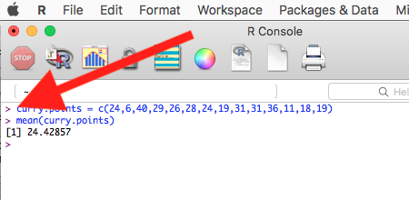
Figure 1. The R GUI on a macOS system; red arrow points to the R prompt.
Everything that exists is an object
.
A brief programmer’s note — John M. Chambers, creator of the S programming language and a member of the R-project team, once wrote that sub-header phrase about R and objects. What that means for us: programming objects can be a combination of variables, functions, and data structures. During an R session the user creates and uses objects. The ls() function is a useful R command to list objects in memory. If you have been following along with your own installed R app, then how many objects are currently available in your session of R? Answer by submitting ls(). Hint: the answer should be one object.
A routine task during analysis is to calculate an estimate then use the result in subsequent work. For example, instead of simply printing the result of mean(curry.points), we can assign the result to an object.
myResult <- mean(curry.points)
.
To confirm the new object was created, try ls() again. And, of course, there’s no particular reason to use the object name, myResult, I provided! Like any programming language, creating good object names will make your code easier to understand.
When you submit the above code, R returns the prompt, and the result of the function call is not displayed. View the result by submitting the object’s name at the R prompt, in this case, myResult. Alternatively, a simple trick is to string commands on the same line by adding ; (semicolon) at the end of the first command. For example,
myResult <- mean(curry.points); myResult
.
Write your code as script
.
While it is possible to submit code one line at a time, a much better approach is to create and manage code in a script file. A script file is just a text file with one command per line, but potentially containing many lines of code. Script files help automate R sessions. Once the code is ready, the user submits code to R from the script file.
Note: Working with scripts eliminates the R prompt, but code is still interpreted one line at a time. The user does not type the prompt in a script file.
Figure 2 shows how to create a new script file via the RGUI menu: File → New script.
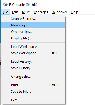
Figure 2. Screenshot of drop down menu RGUI, create new script, Windows 10.
The default text editor opens (Fig 3).
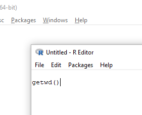
Figure 3. Screenshot of portion of R Script editor, Windows 11. A simple R command is visible.
Submit code by placing cursor at start of the code or, if code consists of multiple lines, select all of the code, then hit keyboard keys Ctrl+R (Windows 11) or for macOS, Cmd+Enter.
By default, save R script files for reuse with the file extension .R, e.g., myScript.R. Because the scripts are just text files you can use other editors that may make coding more enjoyable (see RStudio in particular, but there are many alternatives, some free to use. A good alternative is ESS).
Install R Commander package
.
By now, you have installed the base package of the R statistical programming language. The base package contains all of the components you would need to create and run data analysis and statistics on sets of data. However, you would quickly run into the need to develop functions, to write your own programs to facilitate your work. One of the great things about R is that a large community of programmers have written and contributed their own code; chances are high that someone has already written a function you would need. These functions are submitted in the form of packages. Throughout the semester we will install several R packages to extend R capabilities. R packages discussed in this book are listed at R packages of the Appendix.
Our first package to install is R Commander, Rcmdr for short. R Commander is a package that adds function to R; it provides a familiar point-and-click interface to R, which allows the user to access functions via a drop-down menu system (Fox 2017). Thus, instead of writing code to run a statistical test, Rcmdr provides a simple menu driven approach to help students select and apply the correct statistical test. R Commander also provides access to Rmarkdown and a menu approach to rendering reports.
install.packages("Rcmdr")
.
In addition, download and install the plugin
install.packages("RcmdrMisc")
See Install R Commander for detailed installation instructions.
Plugins are additional software which add function to an existing application.
Start R Commander
.
After installing Rcmdr, to start R Commander, type library(Rcmdr) at the R prompt and enter to load the library
library(Rcmdr).
On first run of R Commander you may see instructions for installing additional packages needed by R Commander. Accept the defaults and proceed to complete the installation of R Commander. Next time you start R commander the start up will be much faster since the additional packages needed by R Commander will already be present on your computer.
Note that you don’t type the R prompt and, indeed, in R Commander Script window you won’t see the prompt (Fig 4). Instead, you enter code in the R Script window, then click “Submit” button (or Win11: Ctrl+R or for macOS: Cmd+Enter), to send the command to the R interpreter. Results are sent to Output window (Fig 4).
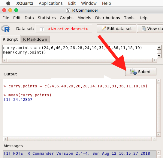
Figure 4. The windows of R Commander, macOS. From bottom to top: Messages, Output, Script (tab, Markdown) Rcmdr ver. 2.4-4.
Figure 4 shows how the R Commander GUI looks on a macOS computer. The look is similar on Microsoft Windows 11 machines (Fig 5).
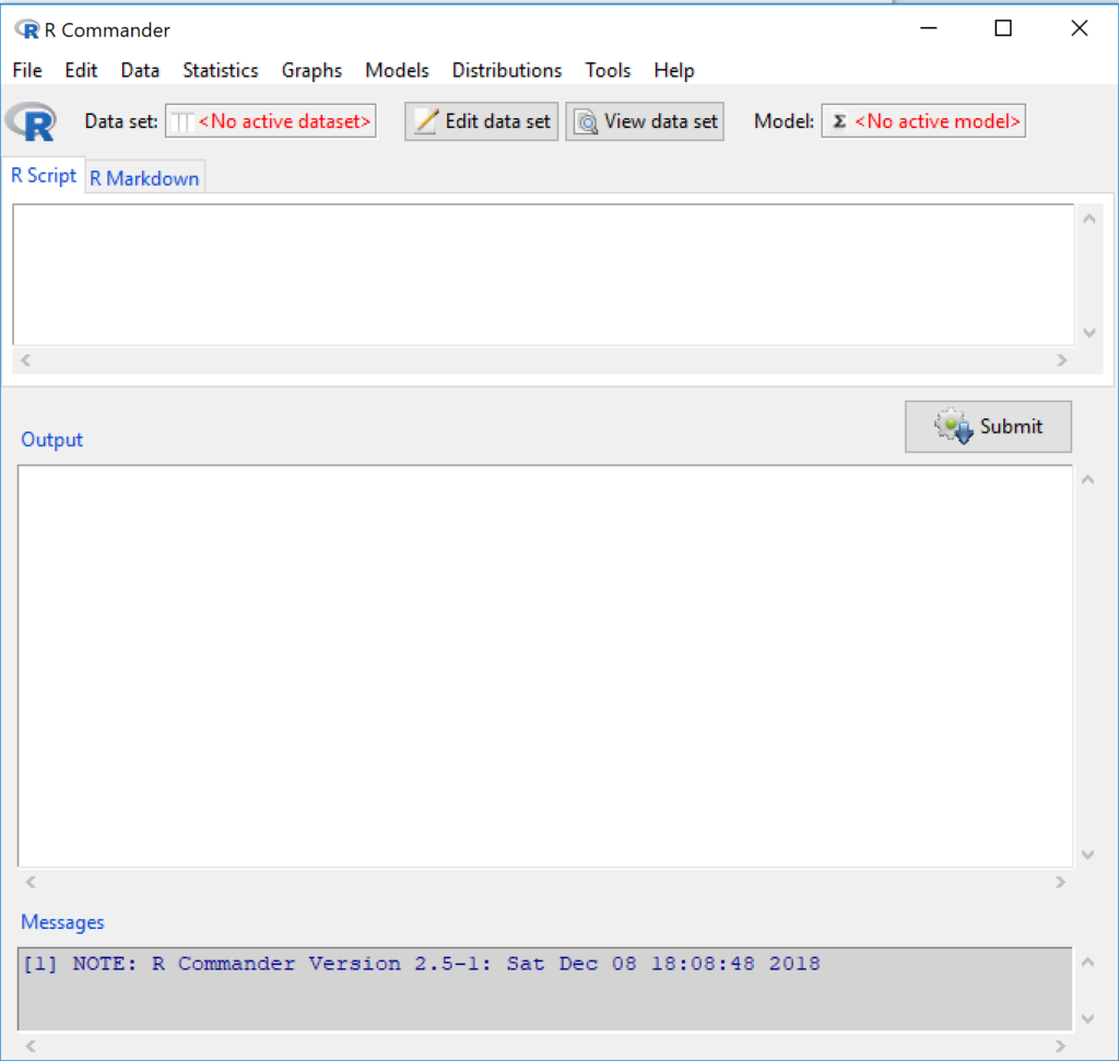
Figure 5. The windows of R Commander, Win11. From bottom to top: Messages, Output, Script (tab, R Markdown) Rcmdr ver. 2.5-1.
We use R Commander because it gives us access to code from drop-down menus, which at least initially, helps learn R (Fox 2005, Fox 2016). Later, you’ll want to write the code your self, and RStudio provides a nice environment to accomplish your data analysis.
Improve Rcmdr experience. After installing R and Rcdmr, Win11 users should change from MDI to SDI — one big window to separate windows, respectively (see Do explore settings, Figure 5). macOS users should turn off Apple’s app nap (see Do explore settings, Figures 6 & 7), which should improve a Mac user’s experience with R Commander and other X Window applications.
Complete R setup by installing LaTeX and pandoc for Markdown
.
LaTeX is a system for document preparation. pandoc is a document converter system. Markdown is a language used to create formatted writing from simple text code. Once these supporting apps are installed, sophisticated reports can be generated from R sessions, by-passing copy and paste methods one might employ. See Install R Commander for instructions to add these apps.
Note: If you successfully installed R and are running R Commander, but may be having problems installing pandoc or LaTeX, then this note is for you. While there’s advantages to getting pandoc etc working, it is not essential for BI311 work.
Assuming you have Rcmdr and RcmdrMisc installed, and if you have started Rcmdr and have it up and running, then we can skip pandoc and LaTeX installation and use features of your browser to save to pdf.
R Markdown by default will print to a web page (an html document called RcmdrMarkdown.html) and display it in your default browser. To meet requirements of BI311 — you submit pdf files — we can print the html document generated from “Generate Report” in R Commander to a pdf.
- Chrome browser, right click in the web page, from the popup menu select Print, then change destination to Save as pdf.
- Safari browser, right click then select Print page (or if an option, Save page as pdf), then find at lower left find PDF and option to Save as PDF.
R Markdown
.
Markdown is a syntax for plain text formatting and is really helpful for generating clean html (web) files. R Commander also helps us with our reporting. R Markdown is provided as a tab (Fig 4, 5). Provided you have also installed pandoc on your computer, you can also convert or “render” the work into other formats including pdf and epub. Unsure if your computer has pandoc installed? If you are unsure than most likely it is not installed. 😁 Rcmdr provides a quick check — go to Tools and if you see Install auxiliary software, then click on it and a link to pandoc website to find and download installation file. You can also confirm install of pandoc by opening a terminal on your computer (e.g., search “terminal” on macOS or “cmd” on Win11), then enter pandoc –version at the shell prompt. Figure 6 shows version pandoc is installed on my Win11 HP laptop.
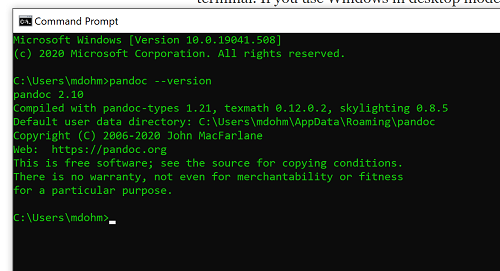
Figure 6. Screenshot of terminal window (cmd) on win11 computer, checking for installed pandoc on a win10 pc.
Enter your R code in the script window, submit your code, and your results (code, output, graphs) are neatly formatted for you by Markdown. Once the Markdown file is created in R Commander, you can then export to an html file for a a web browser, an MS Word document, or other modes.
Do explore settings!
.
After installation, R and R Commander are ready to go. However, students are advised that a few settings may need to be changed to improve performance. For example, on Win11 PCs, R Commander recommends changing from the default MDI (Multiple Document Interface) to SDI (Single Document Interface). Check the SDI button via Edit menu, select GUI preferences menu. Click save, which will make changes to .RProfile, then exit and restart R. Check to make sure the changes have been made (Fig 7).
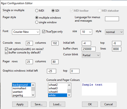
Figure 7. Screenshot of GUI preferences settings after changing from default MDI to SDI, win10
For macOS users, both R and Rcmdr will run better if you turn off Apple’s power saving feature called nap. From Rcmdr go to Tools and select Manage Mac OS X app nap for R.app… (Fig 8).
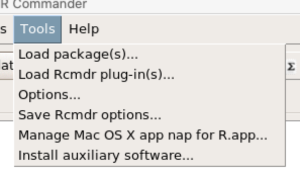
Figure 8. Screenshot Rcmdr Tools popup menu, macOS 10.15.6
A dialog box appears; select off to turn off app nap (Fig 9).
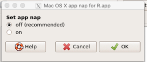
Figure 9. Screenshot Rcmdr Set app nap dialog box, macOS 10.15.6
Exit R Commander
.
Click on Rcmdr: File → Exit, then choose to exit from just R Commander, or both R Commander and R.
If you exit just R Commander or both R and R Commander, you’ll receive a pop-up request to confirm you want to quit R Commander (click yes), and a second prompt asking if you want to save your script. In general, select yes and then you’ll be able to take up where you left off. Similarly, if asked to save your workspace, choose no. If you save workspace, this creates an .RProfile text file with settings for how R and R Commander will behave the next time you start R. The file will be saved to your current working folder, which R will use the next time R starts. At least while you are getting started, you should avoid creating these .RProfile files.
As long as the current session of R is active, then the library for Rcmdr, as well as any other library loaded during the R session, is in memory. To start R Commander again while R is running, at the R prompt, type and submit
Commander()
.
Questions
.
- Biostatistics students should work through my ten R lessons, A quick look t R and R Commander, available in Mike’s Workbook for Biostatistics.
- Students should also search Internet for R tutorials and R Commander tutorials. Find recent tutorials and work through several of them. We get better when we practice.
Chapter 1 contents
.
- Getting started
- A quick look at R and R Commander
- Chapter 1 – References