13.1 – ANOVA Assumptions
Introduction
Like all parametric tests, assumptions are made about the data in order to justify and trust estimates and inferences drawn from ANOVA. While acknowledging the “experimental design” message suggested by the xkcd panel in Figure 1 — the presence of a large effect size between groups mitigates the technical necessities of inferential statistics — of course, not all of our projects will have such obvious results. Understanding the impact of assumptions on inference is a key concept in (bio)statistics: when the p-value is close to the Type I error rate, deviations from assumptions may reduce our confidence in the “statistical significance” of the result.

Figure 1. xkcd.com “Statistics,” https://xkcd.com/2400/.
ANOVA assumptions include:
- Data come from normal distributed population. View with a histogram or Q-Q plot. Test with Shapiro-Wilks or other appropriate goodness of fit test (see Question 1 below). Normality tests are the subject of Chapter 13.3.
- Sample size equal among groups.
- This is an example of a potentially confounding factor — If sample sizes differ, then any difference in means could be simply because of differences in sample size! This gets us into weighted versus unweighted means.
- You shouldn’t be surprised that modern implementations of ANOVA in software easily handle (adjust for) these known confounding factors. Depending on the program, you’ll see “Adjusted means,” “least squares means,” “Marginal means” etc. This just implies that the group means are compared after accounting for confounding factors.
- Importantly, as long as sample sizes among the groups are roughly equivalent, normality assumption is not a big deal (low impact on risk of Type I error).
- Independence of errors. One consequence of this assumption is that you would not view 100 repeated observations of a trait on the same subject as 100 independent data points. We’ll return to this concept more in the next two lectures. Some examples:
-
- Colorimetric assay where the signal changes over time, and you measure in order (eg, samples from group 1 first, samples from group 2 second, etc.) — this confounds group with time.
- The consequence is that you are far more likely to reject the null hypothesis, committing a Type I error.
- Let’s say you are observing running speeds of ten mongoose. However, it turns out that five of your subjects are actually from the same family, identical quintuplets! Do you really have ten subjects?
- Compare brain-body mass ratio among different species; this is a classic comparative method problem (Fig. 3). Since 1985 (Felsenstein 1985), it was recognized that the hierarchical evolutionary relationships among the species must be accounted for to control for lack of independence among the taxa tested. See Phylogenetically independent contrasts, Chapter 20.12.
- Colorimetric assay where the signal changes over time, and you measure in order (eg, samples from group 1 first, samples from group 2 second, etc.) — this confounds group with time.
- Equal variances (homogeneity) among groups. See Chapter 13.4 for how to test this for multiple groups.
Impact of assumptions
R — and pretty much all statistics packages — will calculate the ANOVA table and the p-value, but it is up to you to recognize that the P-value is accurate only if the assumptions are met. Violation of the assumption of normality can lead to Type I errors occurring more often than the 5% level. What to do if the assumptions are violated?
If the violation is due to only a handful of the data, you might proceed anyway. But following a significant test for normality, we could avoid the ANOVA in favor of nonparametric alternatives (Chapter 15), or, we might try to transform the data.
Consider a histogram of brains weight measures in grams for a variety of mammals (Fig 2).
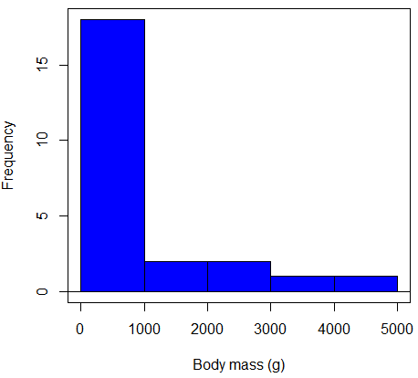
Figure 2. Histogram of body mass (g) for 24 mammals (data from Boddy et al 2012).
We will introduce a variety of statistical tests of the assumption of normality in Chapter 13.3, but looking at a histogram as part of our data exploration, we clearly see the data are right-skewed (Fig 2). Is this an example of normal distributed sample of observations? Clearly not. If we proceed with statistical tests on the raw data set, then we are more likely to commit a Type I error (ie, we will reject the null hypothesis more often than we should).
A comment on normality and biology. It is very possible that data may not be normally distributed or have equal variances on the original scale, but a simple mathematical manipulation may take care of that. In fact, in many case in biology that involve growth, many types of variables are expected to not be normal on the original scale. For example, while the relationship between body mass,  , and metabolic rate,
  , in many groups of organisms is allometric and increases positively, the relationship

is not directly proportional (linear) on the original scale. By taking the logarithm of both body mass and metabolic rate, however, the relationship is linear

In fact, taking the logarithm (base 10, base 2, or base e) is often a common solution to both non-normal data (Fig 2) and unequal variances.
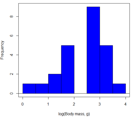
Figure 3. Histogram of log10-transformed body mass observations from Figure 2.
Other common transformations include taking the square root or the inverse of the square-root for skewed or kurtotic sample distributions, and the arcsine for frequencies (since frequencies can only be from 0 to 1 — need to “stretch the data” to make frequencies fit procedures like ANOVA). There are many issues about data transformation, but keep in mind three points. After completing the transformation, you should check the assumptions (normality, equal variances) again.
You may need to recode the data before applying a transform. For example, you cannot take the square root or logarithm of negative numbers. If you do not recode the data, then you will lose these observations in your subsequent analyses. In many cases, this problem is easily solved by adding 1 to all data points before making the transform. I prefer to make the minimum value 1 and go from there. The justification for data transformation is basically to realize that there is no necessity to use the common arithmetic or linear scale: many relationships are multiplicative or nonadditive (eg, rates in biology and medicine).
Note 1: Instead of transformations or other ad hoc manipulations of the data, modern statistical approaches favor modeling the error structure of the data within a Generalized Linear Model framework (St.-Pierre et al 2018). The advantage of the model approach is that parameter estimation occurs on the raw data. Use of transformations may, however, remain a better choice. While statistically justified, the generalized linear model approach may also tend to have higher rates of Type II error compared to simple transformations.
Statistical outlier
Another topic we should at least mention here is the concept of outliers. While most observations tend to cluster around the mean or middle of the sample distribution, occasionally one or more observations may differ substantially from the others. Such values are called outliers, and we note that there are two possible explanations for an outlier
- the value could be an error.
- it is a true value.
Note 2: “it is a true value,” and there may be an interesting biological explanation for its cause, ie, extraordinary individuals.
We encountered a clear outlier in the BMI homework. If the reason is (1), then we go back and either fix the error or delete it from the worksheet. If (2), however, then we have no objective reason to exclude the point from our analyses.
We worry if the outlier influences our conclusions — so it is a good idea to run your analyses with and without the outlier. If your conclusions remain the same, then no worries. If your conclusions change based on one observation, then this is problematic. For the most part you are then obligated to include the outlier and the more conservative interpretation of your statistical tests.
ANOVA is robust to modest deviations from assumptions
A comment about ANOVA assumptions ANOVA turns out to be robust to violations of item (1) or (2). That means unless the data are really skewed or the group sizes are very different, ANOVA will perform well (Type I error rate stays close to the specified 5% level). We worry about this however when p-value is very close to alpha!!
The third assumption is more important in ANOVA.
Like the t-test, ANOVA makes the assumption of equal variances among the groups, so it will be helpful to review why this assumption is important to both the t-test and ANOVA. In the two-sample independent t-test, the pooled sample variance,  , is taken as an estimate of the population variance,
  . If you recall,
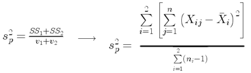
where  refers to the sum of squares for the first group and
  refers to the second group sum of squares (see our discussion on measures of dispersion) and
  refers to the degrees of freedom for the first group and
  refers to the second group degrees of freedom. We make a similar assumption in ANOVA. We assume that the variances for each sample are the same and therefore that they all estimate the population variance . To say it in another way, we are assuming that all of our samples have identical variability
Once we make this assumption, we may pool (or combine) all of the SSs and DFs for all groups as our best estimate of the population variance, . The trick to understanding ANOVA is to realize that there can be two types of variability: there is variability due to being part of a group (e.g., even though ten human subjects receive the same calorie-restricted diet, not all ten will loose the same amount of weight) and there is variability among or between groups (e.g., on average, all subjects who received the calorie-restricted diet lost more weight than did those subjects who were on the non-restricted diet).
Example
The encephalization index (or encephalization quotient) is defined as the ratio of size the brain compared to body size. While there is a well-recognized increase in brain size given increased body size, encephalization describes a shift of function to cortex (frontal, occipital, parietal, temporal) from noncortical parts of the brain (cerebellum, brainstem). Increased cortex is associated with increased complexity of brain function; for some researchers, the index is taken as a crude estimate of intelligence. Figure 4A shows plot of brain mass in grams versus body size (grams) for 24 mammal species (data sampled from Boddy et al 2012); Figure 4B shows the same data, but following log10-transform of both variables.
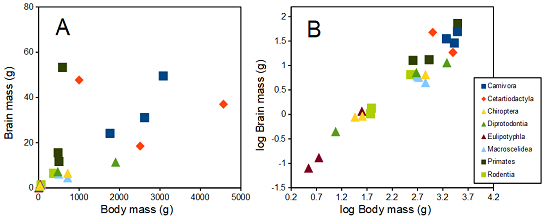
Figure 4. Plot of brain and body weights (A) and log10-log10 transform (B) for a variety of species (data from Boddy et al 2012). The ratio is called encephalization index.
Looking at the two figures the linear relationship between the two variables is obvious in Figure 4B, less so for Figure 4A. Thus, one biological justification for transformation of the raw data is exemplified with the brain-body mass dataset: the association is allometric not additive. The other reason to apply a transform is statistical; the log10-transform improves the normality of the variables. Take a look at the Q-Q plot for the raw data (Fig 5) and for the log10-transformed data (Fig 6).
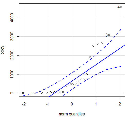
Figure 5. Q-Q plot, body mass, raw data. Compare to Figure 2.
Figure 5 is a good test of your observation skills — what are you supposed to look for in a Q-Q plot? Follow the dots — the data don’t fall on the straight line. A few even fall outside of the confidence interval (the curved dashed lines), which suggests the data were not normally distributed (see histogram, Fig 2). And for the transformed data, the Q-Q plot is shown in Figure 6.
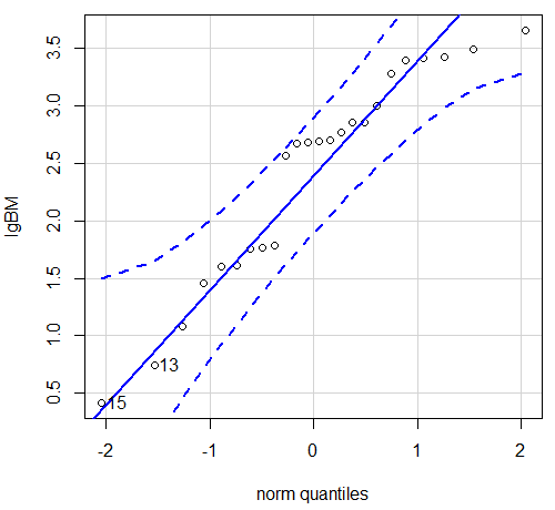
Figure 6. Q-Q plot same data, log10-transformed, compare to Figure 2.
Compared to the raw data, the transformed data now fall on the line and none are outside of the confidence interval. We would conclude that the transformed data are more normal, thus, better meeting the assumptions of our parametric tests.
Lack of independence among data
Species comparisons are common in evolutionary biology and related fields. As noted earlier, comparative data should not be treated as independent data points (discussed in 20.12 – Phylogenetically independent contrasts). For our 24 species, I plotted the estimate of the phylogeny (timetree.org), represented in Figure 7. Some species are closely related (eg the two elephant shrews, Rhynchocyon genus). Thus, because of the hierarchical, nested nature of evolution — first articulated by Charles Darwin — instead of 24 independent data points, we have eight clusters of points (see Question 4).
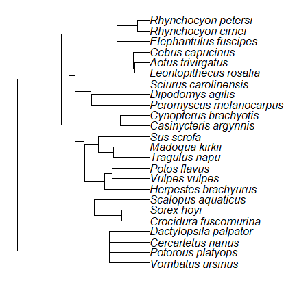
Figure 7. Phylogenetic tree of 24 species used in this report.
Note 3: The relevant quote from Charles Darwin: “… the inevitable result is that the modified descendants proceeding from one progenitor become broken up into groups subordinate to groups,” and was illustrated by the only figure in Origin of Species (both quote and illustration are in Chapter 4).
The conclusion? We don’t have 24 data points, more like 8 points. Because the species are more or less related, there are fewer than 24 independent data points. Statistically, this would mean that the errors are correlated. Various approaches to account for this lack of independence have been developed; perhaps the most common approach is to apply phylogenetically independent contrasts, a topic discussed in Chapter 20.12. (Boddy et al 2012 used this approach.)
Note 4: See 20.11 – Plot a Newick tree for how to plot phylogeny trees in R.
Questions
- Make a histogram for the brain mass data set.
- Shapiro-Wilks is one test of normality.
- Can you recall the name of the other normality tests we named?
- Run tests of normality on both body mass and brain mass data. Interpret the results, frame your response with keywords: “central tendency,” “outliers,” “shape,” and “symmetry.”
- Calculate moment statistics for the body mass and brain mass data set, both raw and log10-transformed data. Interpret your results, taking care to frame your answer with the following keywords: “shape,” “symmetry,” and “peakedness” (aka “tailedness”).
- We introduced the lack of independence for comparative data attributed to the evolutionary process. Statistically, the impact is on degrees of freedom; for example, if we ignore the lack of independence in the data set, df = 22 for the slope coefficient in a linear regression. However, given the degrees of freedom would be closer to six! What are the effects on Type I error rate of lack of independence?
Quiz Chapter 13.1
ANOVA assumptions
Data set and R code used in this page
species, order, body, brain
'Herpestes ichneumon', Carnivora, 1764, 24.1
'Potos flavus', Carnivora, 2620, 31.05
'Vulpes vulpes', Carnivora, 3080, 49.5
'Madoqua kirkii', Cetartiodactyla, 4570, 37
'Sus scrofa', Cetartiodactyla, 1000, 47.7
'Tragulus napu', Cetartiodactyla, 2510, 18.5
'Casinycteris argynnis', Chiroptera, 40.5, 0.92
'Cynopterus brachyotis', Chiroptera, 29, 0.88
'Potorous platyops', Chiroptera, 718, 6.5
'Cercartetus nanus', Diprotodontia, 12, 0.44548
'Dactylopsila palpator', Diprotodontia, 474, 7.15876
'Vombatus ursinus', Diprotodontia, 1902, 11.396
'Crocidura fuscomurina', Eulipotyphla, 5.6, 0.13
'Scalopus aquaticus', Eulipotyphla, 39.6, 1.48
'Sorex hoyi', Eulipotyphla, 2.6, 0.107
'Elephantulus fuscipes', Macroscelidea, 57, 1.33
'Rhynchocyon cirnei', Macroscelidea, 490, 6.1
'Rhynchocyon petersi', Macroscelidea, 717.3, 4.46
'Aotus trivirgatus', Primates, 480, 15.5
'Cebus capucinus', Primates, 590, 53.28
'Leontopithecus rosalia', Primates, 502.5, 11.7
'Dipodomys agilis', Rodentia, 61.4, 1.34
'Peromyscus melanocarpus', Rodentia, 58.8, 1.03
'Sciurus carolinensis', Rodentia, 367, 6.49
The Newick code for the tree in Figure 6.
((Vombatus_ursinus:48.94499077,((Potorous_platyops:47.59556667,Cercartetus_nanus:47.59556667)'14':0.66887333,Dactylopsila_palpator:48.26444000)'13':0.68055077)'11':109.65259681,(((((Crocidura_fuscomurina:33.74066667,Sorex_hoyi:33.74066667)'10':33.03022424,Scalopus_aquaticus:66.77089091)'19':22.55292749,(((Herpestes_brachyurus:54.32144118,(Vulpes_vulpes:45.52834967,Potos_flavus:45.52834967)'9':8.79309151)'22':23.43351523,((Tragulus_napu:43.96862857,Madoqua_kirkii:43.96862857)'8':17.99735995,Sus_scrofa:61.96598852)'6':15.78896789)'30':0.77378567,(Casinycteris_argynnis:35.20000000,Cynopterus_brachyotis:35.20000000)'29':43.32874208)'27':10.79507632)'35':7.13857077,(((Peromyscus_melanocarpus:69.89837667,Dipodomys_agilis:69.89837667)'43':0.64655123,Sciurus_carolinensis:70.54492789)'42':19.27825952,((Leontopithecus_rosalia:18.38385647,Aotus_trivirgatus:18.38385647)'40':1.29720005,Cebus_capucinus:19.68105652)'48':70.14213090)'51':6.63920175)'47':8.99739162,(Elephantulus_fuscipes:39.23366667,(Rhynchocyon_cirnei:15.34500000,Rhynchocyon_petersi:15.34500000)'39':23.88866667)'56':66.22611412)'55':53.13780679);