19.1 – Jackknife sampling
Introduction
edits: — under construction —
R packages
There are several R packages one could use. The package bootstrap may be the the most general, and includes a jackknife routine suitable for any function. This page demonstrates jackknife estimate of correlation.
Example data set, cars, stopping distance by speed of car (scroll down or click here).
install package bootstrap
Jackknife estimates on linear models
These procedures can be done with the bootstrap package, but lmboot is a specific package to solve the problem
install package lmboot
Example data set, Tadpoles from Chapter 14, copied to end of this page for your convenience (scroll down or click here).
R code
jackknife(VO2~Body.mass, data = Tadpoles)
R returns two values:
bootEstParam, which are the jackknife parameter estimates. Each column in the matrix lists the values for a coefficient. For this model,bootEstParam$[,1]is the intercept andbootEstParam$[,2]is the slope.origEstParam, a vector with the original parameter estimates for the model coefficients.
$bootEstParam
     (Intercept) Body.mass
[1,]   -660.8403  472.6841
[2,]   -539.5951  430.3990
[3,]   -612.8495  454.5188
[4,]   -512.5914  423.0815
[5,]   -543.1577  434.2789
[6,]   -572.3895  442.9176
[7,]   -613.7873  451.2656
[8,]   -594.0366  446.2571
[9,]   -582.1833  443.5404
[10,]  -598.2244  456.0599
[11,]  -531.3152  415.2467
[12,]  -555.7287  430.5604
[13,]  -726.8522  512.1268

$origEstParam
[,1]
(Intercept) -583.0454
Body.mass 444.9512
Get necessary statistics and plots
#95% CI slope
quantile(jack.model.1$bootEstParam[,2], probs=c(.025, .975))
R returns
    2.5%    97.5%
417.5971 500.2940
#95% CI intercept
quantile(jack.model.1$bootEstParam[,1], probs=c(.025, .975))
R returns
     2.5%     97.5%
-707.0486 -518.2085
Coefficient estimates
Slope
#plot the sampling distribution of the slope coefficient
par(mar=c(5,5,5,5)) #setting margins to my preferred values
hist(jack.model.1$bootEstParam[,2], col="blue", main="Jackknife Sampling Distribution",
xlab="Slope Estimate")
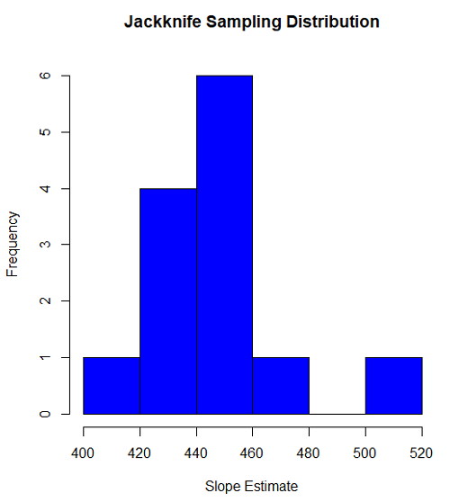
Figure 1. histogram of jackknife estimates for slope
Intercept
#95% CI intercept
quantile(jack.model.1$bootEstParam[,1], probs=c(.025, .975))
par(mar=c(5,5,5,5))
hist(jack.model.1$bootEstParam[,1], col="blue", main="Jackknife Sampling Distribution",
xlab="Intercept Estimate")
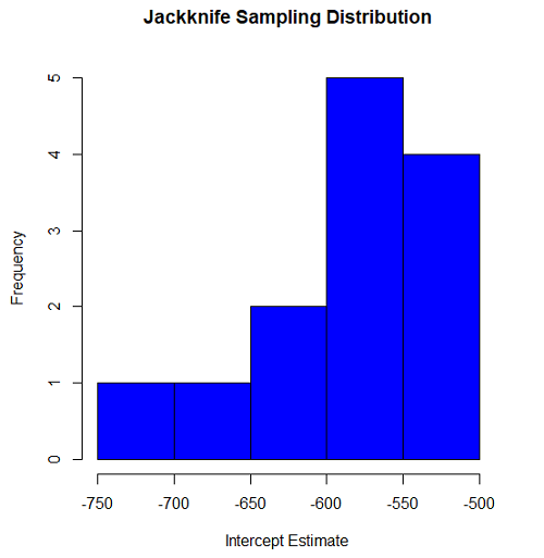
Figure 2. Histogram of jackknife estimates for intercept.
Questions
edits: pending
cars data set used this page
| speed | dist |
| 4 | 2 |
| 4 | 10 |
| 7 | 4 |
| 7 | 22 |
| 8 | 16 |
| 9 | 10 |
| 10 | 18 |
| 10 | 26 |
| 10 | 34 |
| 11 | 17 |
| 11 | 28 |
| 12 | 14 |
| 12 | 20 |
| 12 | 24 |
| 12 | 28 |
| 13 | 26 |
| 13 | 34 |
| 13 | 34 |
| 13 | 46 |
| 14 | 26 |
| 14 | 36 |
| 14 | 60 |
| 14 | 80 |
| 15 | 20 |
| 15 | 26 |
| 15 | 54 |
| 16 | 32 |
| 16 | 40 |
| 17 | 32 |
| 17 | 40 |
| 17 | 50 |
| 18 | 42 |
| 18 | 56 |
| 18 | 76 |
| 18 | 84 |
| 19 | 36 |
| 19 | 46 |
| 19 | 68 |
| 20 | 32 |
| 20 | 48 |
| 20 | 52 |
| 20 | 56 |
| 20 | 64 |
| 22 | 66 |
| 23 | 54 |
| 24 | 70 |
| 24 | 92 |
| 24 | 93 |
| 24 | 120 |
| 25 | 85 |
Data set used this page (sorted)
| Gosner | Body mass | VO2 |
| I | 1.76 | 109.41 |
| I | 1.88 | 329.06 |
| I | 1.95 | 82.35 |
| I | 2.13 | 198 |
| I | 2.26 | 607.7 |
| II | 2.28 | 362.71 |
| II | 2.35 | 556.6 |
| II | 2.62 | 612.93 |
| II | 2.77 | 514.02 |
| II | 2.97 | 961.01 |
| II | 3.14 | 892.41 |
| II | 3.79 | 976.97 |
| NA | 1.46 | 170.91 |
Chapter 19 contents
- Introduction
- Jackknife sampling
- Bootstrap sampling
- Ch19 References and suggested readings