7.4 – Epidemiology: Relative risk and absolute risk, explained
Risk communication.
Epidemiology is the study of patterns of health and illness of populations. An important task in an epidemiology study is to identify risks associated with disease. Epidemiology is a crucial discipline used to inform about possible effective treatment approaches, health policy, and about the etiology of disease.
Please review terms presented in section 7.1 before proceeding. RR and AR are appropriate for cohort-control and cross-sectional studies (see 2.4 and 5.4) where base rates of exposure and unexposed or numbers of affected and non-affected individuals (prevalence) are available. Calculations of relative risk (RR) and relative risk reduction (RRR) are specific to the sampled groups under study whereas absolute risk (AR) and absolute risk reduction (ARR) pertain to the reference population. Relative risks are specific to the study, absolute risks are generalized to the population. Number needed to treat (NNT) is a way to communicate absolute risk reductions.
An example of ARR and RRR risk calculations using natural numbers.
Clinical trials are perhaps the essential research approach (Sibbald and Roland 1998; Sylvester et al 2017); they are often characterized with a binary outcome. Subjects either get better or they do not. There are many ways to represent risk of a particular outcome, but where possible, using natural numbers is generally preferred as a means of communication, particularly to the general public. Consider the following example (pp 34-35, Gigerenzer 2015): What is the benefit of taking a cholesterol-lowering drug, Pravastatin, on the risk of deaths by heart attacks and other causes of mortality? Press releases (e.g., Maugh 1995), from the study stated the following:
“… the drug pravastatin reduced … deaths from all causes 22%”
A subsequent report (Skolbekken 1998) presented the following numbers (Table 1).
Table 1. Reduction in total mortality (5 year study) for people who took Pravastatin compared to those who took placebo.
| Deaths per 1000 people with high cholesterol (> 240 mg/dL) |
No deaths | Cumulative incidence |
||
| Treatment | Pravastatin
(n = 3302) |
a= 32 |
b= 3270 |
CIe |
| Placebo
(n = 3293) |
c= 41 |
d= 3252 |
CIu | |
where cumulative incidence refers to the number of new events or cases of disease divided by the total number of individuals in the population at risk.
Do the calculations of risk
The risk reduction (RR), or the number of people who die without treatment (placebo) minus those who die with treatment (Pravastatin), 

and the cumulative incidence in the exposed (treated) group, CIe, is  , and cumulative incidence in the unexposed (control) group, CIu, is
  . We can calculate another statistic called the risk ratio,

because the risk ratio is less than one, we interpret that statins reduce the risk of mortality from heart attack. In other words, statins lowered the risk by 0.78.
But is this risk reduction meaningful?
Now, consider the absolute risk reduction (ARR) is 
Relative risk reduction, or the absolute risk reduction divided by the proportion of patients who die without treatment, is 
Conclusion: high cholesterol may contribute to increased risk of mortality, but the rate is very low in the population as a whole (the ARR).
Another useful way to communicate benefit is to calculate the Number Needed to Treat (NNT), or the number of people who must receive the treatment to save (benefit) one person. The ideal NNT is a value of one (1), which would be interpreted as everyone improves who receives the treatment. By definition, NNT must be positive; however, a resulting negative NNT would suggest the treatment may cause harm, i.e., number needed to harm (NNH).
For this example, the NNT is

therefore, to benefit one person, 111 need to be treated. The flip side of the implications of NNT, although one person may benefit by taking the treatment, 110 ( ) will take the treatment, but will NOT RECEIVE THE BENEFIT, but do potentially get any side effect of the treatment.
Confidence interval for NNT is derived from the Confidence interval for ARR.
For a sample of 100 people drawn at random from a population (which may number in the millions), then repeat the NNT calculation for a different sample of 100 people, do we expect the first and second NNT estimates to be exactly the same number? No, but we do expect them to be close and we can define what we mean by close as we expect each estimate to be within certain limits. While we expect the second calculation to be close to the first estimate, we would be surprised if it was exactly the same. And so, which is the correct estimate, the first or the second? They both are, in the sense that they both estimate the parameter NNT (a property of a population).
We use confidence interval to communicate where we believe the true estimate for NNT to be. Confidence Intervals (CI) allow us to assign a probability to how certain we are about the statistic and whether it is likely to be close to the true value (Altman 1998, Bender 2001). We will calculate the 95% CI for the ARR using the Wald method, then take the inverse of these estimates for our 95% CI. The Wald method assumes normality.
For CI of ARR, we need sample size for control and treatment groups; like all confidence intervals, we need to calculate the standard error of the statistic, in this, case, the standard error (SE) for ARR is approximately

where SE is the standard error for ARR. For our example, we have

The 95% CI for ARR is approximately 
For the Wald estimate, replace the 2 with  , which comes from the normal table for z at
(why the 2 in the equation? Because it is plus or minus so we divide the frequency 0.95 in half) and for our example, we have 
and the inverse for NNT CI is 
Our example exemplifies the limitation of the Wald approach (cf. Altman 1998): our confidence interval includes zero, and doesn’t even include our best estimate of NNT (111).
Note 1: By now I trust you can see differences for results by direct input of the numbers into R and what you get by the natural numbers approach. In part this is because we round in our natural number calculations — remember, while it makes more sense to communicate about whole numbers (people) and not fractions (fractions of people!), rounding through the calculations adds error to the final value. As long as you know the difference and the relevance between approximate and exact solutions, this shouldn’t cause concern.
Software: epiR.
R has many epidemiology packages, epiR and epitools are two. Most of the code presented stems from epiR.
We need to know about our study design in order to tell the functions which statistics are appropriate to estimate. For our statin example, the design was prospective cohort (i.e., cohort.count in epiR package language), not case-control or cross-sectional (review in Chapter 5.4).
library(epiR)
Table1 <- matrix(c(32,3270,41,3252), 2, 2, byrow=TRUE, dimnames = list(c("Statin", "Placebo"), c("Died", "Lived")))
Table1
        Died Lived
Statin    32  3270
Placebo   41  3252
epi.2by2(Table1, method="cohort.count", outcome = "as.columns")
R output
           Outcome + Outcome - Total           Inc risk *
Exposed +         32      3270  3302 0.97  (0.66 to 1.37)
Exposed -         41      3252  3293 1.25  (0.89 to 1.69)
Total             73      6522  6595 1.11  (0.87 to 1.39)

Point estimates and 95% CIs:
-------------------------------------------------------------------
Inc risk ratio                          0.78 (0.49, 1.23)
Inc odds ratio                          0.78 (0.49, 1.24)
Attrib risk in the exposed *           -0.28 (-0.78, 0.23)
Attrib fraction in the exposed (%)    -28.48 (-103.47, 18.88)
Attrib risk in the population *        -0.14 (-0.59, 0.32)
Attrib fraction in the population (%) -12.48 (-37.60, 8.05)
-------------------------------------------------------------------
Uncorrected chi2 test that OR = 1: chi2(1) = 1.147 Pr>chi2 = 0.284
Fisher exact test that OR = 1: Pr>chi2 = 0.292
Wald confidence limits
CI: confidence interval
* Outcomes per 100 population units
The risk ratio we calculated by hand is shown in green in the R output, along with other useful statistics (see ?epi2x2 for help with these additional terms) not defined in our presentation.
We explain results of chi-square goodness of fit (Ch 9.1) and Fisher exact (Ch 9.5) tests in Chapter 9. Suffice to say here, we interpret the p-value (Pr) = 0.284 and 0.292 to indicate that there is no association between mortality from heart attacks with or without the statin (i.e., the Odds Ratio, OR, not statistically different from one).
Wait! Where’s NNT and other results?
Use another command in epiR package, epi.tests(), to determine the specificity, sensitivity, and positive (or negative) predictive value.
epi.tests(Table1)
and R returns
          Outcome + Outcome - Total
Test +           32      3270  3302
Test -           41      3252  3293
Total            73      6522  6595

Point estimates and 95% CIs:
--------------------------------------------------------------
Apparent prevalence *                    0.50 (0.49, 0.51)
True prevalence *                        0.01 (0.01, 0.01)
Sensitivity *                            0.44 (0.32, 0.56)
Specificity *                            0.50 (0.49, 0.51)
Positive predictive value *              0.01 (0.01, 0.01)
Negative predictive value *              0.99 (0.98, 0.99)
Positive likelihood ratio                0.87 (0.67, 1.13)
Negative likelihood ratio                1.13 (0.92, 1.38)
False T+ proportion for true D- *        0.50 (0.49, 0.51)
False T- proportion for true D+ *        0.56 (0.44, 0.68)
False T+ proportion for T+ *             0.99 (0.99, 0.99)
False T- proportion for T- *             0.01 (0.01, 0.02)
Correctly classified proportion *        0.50 (0.49, 0.51)
--------------------------------------------------------------
* Exact CIs
Additional statistics are available by saving the output from epi2x2() or epitests() to an object, then using summary(). For example save output from epi.2by2(Table1, method="cohort.count", outcome = "as.columns") to object myEpi, then
summary(myEpi)
look for NNT in the R output
$massoc.detail$NNT.strata.wald
       est    lower    upper
1 -362.377 -128.038  436.481
Thus, the NNT was 362 (compared to 111 we got by hand) with 95% Confidence interval between -436 and +128 (make it positive because it is a treatment improvement).
Note 2: Strata (L. layers), refer to subgroups, for example, sex or age categories (see discussion in Ch05.4). Our examples here are not presented as subgroup analysis, but epiR reports by name strata.
epiR reports a lot of additional statistics in the output and for clarity, I have not defined each one, just the basic terms we need for BI311. As always, see help pages (e.g., ?epi.2x2 or ?epitests)for more information about structure of an R command and the output.
We’re good, but we can work the output to make it more useful to us.
Improve output from epiR.
For starters, if we set interpret=TRUE instead of the default, interpret=FALSE, epiR will return a richer response.
fit <- epi.2by2(dat = as.table(Table1), method = "cohort.count", conf.level = 0.95, units = 100, interpret = TRUE, outcome = "as.columns")
fit
R output. In addition to the table of coefficients (above), interpret=TRUE provides more context, shown below
Measures of association strength:
The outcome incidence risk among the exposed was 0.78 (95% CI 0.49 to 1.23) times less than the outcome incidence risk among the unexposed.

The outcome incidence odds among the exposed was 0.78 (95% CI 0.49 to 1.24) times less than the outcome incidence odds among the unexposed.

Measures of effect in the exposed:
Exposure changed the outcome incidence risk in the exposed by -0.28 (95% CI -0.78 to 0.23) per 100 population units. -28.5% of outcomes in the exposed were attributable to exposure (95% CI -103.5% to 18.9%).

Number needed to treat for benefit (NNTB) and harm (NNTH):
The number needed to treat for one subject to be harmed (NNTH) is 362 (NNTH 128 to infinity to NNTB 436).

Measures of effect in the population:
Exposure changed the outcome incidence risk in the population by -0.14 (95% CI -0.59 to 0.32) per 100 population units. -12.5% of outcomes in the population were attributable to exposure (95% CI -37.6% to 8.1%).
That’s quite a bit. Another trick is to get at the table of results. We install a package called broom, which includes a number of ways to handle output from R functions, including those in the epiR package. Broom takes from the TidyVerse environment; tables are stored as tibbles.
library(broom)

# Test statistics
tidy(fit, parameters = "stat")
R output
# A tibble: 3 × 4
term statistic df p.value
<chr> <dbl> <dbl> <dbl>
1 chi2.strata.uncor 1.15 1 0.284
2 chi2.strata.yates 0.909 1 0.340
3 chi2.strata.fisher NA NA 0.292
We can convert the tibbles into our familiar data.frame format, and then select only the statistics we want.
# Measures of association
fitD <- as.data.frame(tidy(fit, parameters = "moa")); fitD
R output, all 15 measures of association!
                  term     estimate     conf.low    conf.high
1       RR.strata.wald    0.7783605    0.4914679   1.23272564
2     RR.strata.taylor    0.7783605    0.4914679   1.23272564
3      RR.strata.score    0.8742994    0.6584540   1.10340173
4       OR.strata.wald    0.7761915    0.4876209   1.23553616
5     OR.strata.cfield    0.7761915           NA           NA
6      OR.strata.score    0.7761915    0.4894450   1.23093168
7        OR.strata.mle    0.7762234    0.4718655   1.26668220
8    ARisk.strata.wald   -0.2759557   -0.7810162   0.22910484
9   ARisk.strata.score   -0.2759557   -0.8000574   0.23482532
10     NNT.strata.wald -362.3770579 -128.0383246 436.48140194
11    NNT.strata.score -362.3770579 -124.9910314 425.84844829
12  AFRisk.strata.wald   -0.2847517   -1.0347210   0.18878949
13  PARisk.strata.wald   -0.1381661   -0.5933541   0.31702189
14  PARisk.strata.piri   -0.1381661   -0.3910629   0.11473067
15 PAFRisk.strata.wald   -0.1248227   -0.3760279   0.08052298
We can call out just the statistics we want from this table by calling to the specific elements in the data.frame (rows, columns).
fitD[c(1,4,7,9,12),]
R output
                 term   estimate   conf.low  conf.high
1      RR.strata.wald  0.7783605  0.4914679  1.2327256
4      OR.strata.wald  0.7761915  0.4876209  1.2355362
7       OR.strata.mle  0.7762234  0.4718655  1.2666822
9  ARisk.strata.score -0.2759557 -0.8000574  0.2348253
12 AFRisk.strata.wald -0.2847517 -1.0347210  0.1887895
Software: epitools.
Another useful R package for epidemiology is epitools, but it comes with it’s own idiosyncrasies. We have introduced the standard 2X2 format, with a, b, c, and d cells defined as in Table 1, above. However, epitools does it differently, and we need to update the matrix. By default, epitools has the unexposed group (control) in the first row and the non-outcome (no disease) is in the first column. To match our a,b,c, and d matrix, use the epitools command to change this arrangement with the rev() argument. Now, the analysis will use the contingency table on the right where the exposed group (treatment) is in the first row and the outcome (disease) is in the first column (h/t M. Bounthavong 2021). Once that’s accomplished, epitools returns what you would expect.
Calculate relative risk
risk1 <- 32 / (3270 + 32)
risk2 <- 41 / (3525 + 41)
risk1 - risk2
and R returns
-0.00180638
odds ratio
library(epitools)
oddsratio.wald(Table1, rev = c("both"))
and R returns
$data
              Outcome
Predictor Disease2 Disease1 Total
 Exposed2      517       36   553
 Exposed1      518       11   529
Total         1035       47  1082

$measure
           odds ratio with 95% C.I.
Predictor   estimate      lower      upper
 Exposed2  1.0000000        NA         NA
 Exposed1  0.3049657 0.1535563  0.6056675

$p.value
two-sided
Predictor  midp.exact  fisher.exact    chi.square
Exposed2           NA            NA            NA
Exposed1 0.0002954494  0.0003001641  0.0003517007
odds ratio highlighted in green.
Software: OpenEpi.
R is fully capable of delivering the calculations you need, but sometimes you just want a quick answer. Online, the OpenEpi tools at https://www.openepi.com/ can be used for homework problems. For example, working with count data in 2 X 2 format, select Counts > 2X2 table from the side menu to bring up the data form (Fig 1).
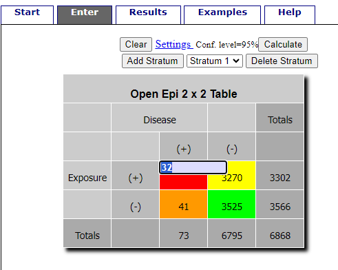
Figure 1. Data entry for 2X2 table at openepi.com.
Once the data are entered, click on the Calculate button to return a suite of results (Fig 2).
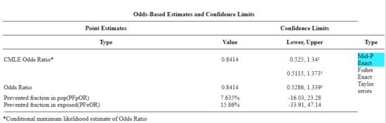
Figure 2. Results for 2X2 table at openepi.com.
Software: RcmdrPlugin.EBM
Note: Fall 2023 — I have not been able to run the EBM plugin successfully! Simply returns an error message — — on data sets which have in the past performed perfectly. Thus, until further notice, do not use the EBM plugin. Instead, use commands in the epiR package.
This isn’t the place nor can I be the author to discuss what evidence based medicine (EBM) entails (cf. Masic et al. 2008), or what its shortcomings may be (Djulbegovic and Guyatt 2017). Rcmdr has a nice plugin, based on the epiR package, that will calculate ARR, RRR and NNT as well as other statistics. The plugin is called RcmdrPlugin.EBM
install.packages("RcmdrPlugin.EBM", dependencies=TRUE)
After acquiring the package, proceed to install the plug-in. Restart Rcmdr, then select Tools and Rcmdr Plugins (Fig 3).
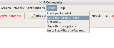
Figure 3. Rcmdr: Tools → Load Rcmdr plugins…
Find the EBM plug-in, then proceed to load the package (Fig 4).
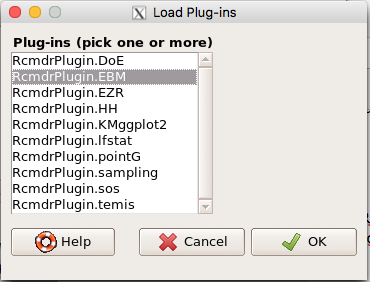
Figure 4. Rcmdr plug-ins available (after first download the files from an R mirror site).
Restart Rcmdr again and the menu “EBM” should be visible in the menu bar. We’re going to enter some data, so choose the Enter two-way table… option in the EBM plug-in (Fig 5)
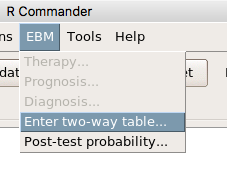
Figure 5. R Commander EBM plug-in, enter 2X2 table menus.
To review, we have the following problem, illustrated with natural numbers and probability tree (Fig 6).
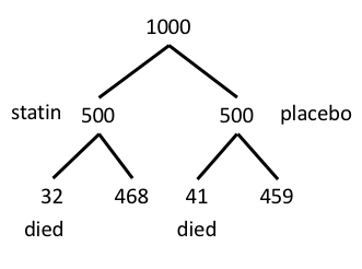
Figure 6. Illustration of probability tree for the statin problem.
Now, let’s enter the data into the EBM plugin. For the data above I entered the counts as
| Lived | Died | |
| Statin | 468 | 32 |
| Placebo | 459 | 41 |
and selected the “Therapy” medical indicator (Fig 7).
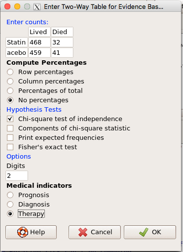
Figure 7. EBM plugin with two-way table completed for the statin problem.
The output from EBM plugin was as follows. I’ve added index numbers in brackets so that we can point to the output that is relevant for our worked example here.
(1) .Table <- matrix(c(468,32,459,41), 2, 2, byrow=TRUE, dimnames = list(c('Drug', 'Placebo'), c('Lived', 'Dead')))
(2) fncEBMCrossTab(.table=.Table, .x='', .y='', .ylab='', .xlab='', .percents='none', .chisq='1', .expected='0', .chisqComp='0', .fisher='0', .indicators='th', .decimals=2)
R output begins by repeating the commands used, here marked by lines (1) and (2). The statistics we want follow in the next several lines of output.
(3) Pearson's Chi-squared test data: .Table X-squared = 1.197, df = 1, p-value = 0.2739
(4) # Notations for calculations Event + Event -Treatment "a" "b" Control "c" "d"
(5)# Absolute risk reduction (ARR) = -1.8 (95% CI -5.02 - 1.42) %. Computed using formula: [c / (c + d)] - [a / (a + b)]
(6)# Relative risk = 1.02 (95% CI 0.98 - 1.06) %. Computed using formula: [c / (c + d)] / [a / (a + b)]
(7)# Odds ratio = 1.31 (95% CI 0.81 - 2.11). Computed using formula: (a / b) / (c / d)
(8) # Number needed to treat = -55.56 (95% CI 70.29 - Inf). Computed using formula: 1 / ARR
9)# Relative risk reduction = -1.96 (95% CI -5.57 - 1.53) %. Computed using formula: { [c / (c + d)] - [a / (a + b)] } / [c / (c + d)]
(10)# To find more about the results, and about how confidence intervals were computed, type ?epi.2by2 . The confidence limits for NNT were computed as 1/ARR confidence limits. The confidence limits for RRR were computed as 1 - RR confidence limits.
end R output
In summary, we found no difference between statin and placebo (P-value = 0.2739) and ARR of -1.8%
Questions.
Data from a case-control study on alcohol use and esophageal cancer (Tuyns et al (1977), example from Gerstman 2014). Cases were men diagnosed with esophageal cancer from a region in France. Controls were selected at random from electoral lists from the same geographical region.
| Esophageal cancer | |||
|
Alcohol grams/day |
Cases | Noncases |
Total |
| > 80 | 96 | 109 |
205 |
|
< 80 |
104 |
666 |
770 |
| Total | 200 | 775 | 975 |
- What was the null hypothesis? Be able to write the hypothesis in symbolic form and as a single sentence.
- What was the alternative hypothesis? Be able to write the hypothesis in symbolic form and as a single sentence.
- What was the observed frequency of subjects with esophageal cancer in this study? And the observed frequency of subjects without esophageal cancer?
- Estimate Relative Risk, Absolute Risk, NNT, and Odds ratio?
- Which is more appropriate, RR or OR? Justify your decision.
- The American College of Obstetricians and Gynecologists recommends that women with an average risk of breast cancer (BC) over 40 get an annual mammogram. Nationally, the sensitivity of mammography is about 68% and specificity of mammography is about 75%. Moreover, mammography involves exposure of women to radiation, which is known to cause mutations. Given that the prevalence of BC in women between 40 and 49 is about 0.1%, please evaluate the value of this recommendation by completing your analysis.
A) In this age group, how many women are expected to develop BC?
B) How many False negative would we expect?
C) How many positive mammograms are likely to be true positives? - “Less than 5% of women with screen-detectable cancers have their lives saved,” (quote from BMC Med Inform Decis Mak. 2009 Apr 2;9:18. doi: 10.1186/1472-6947-9-18): Using the information from question 5, What is the Number Needed to Treat for mammography screening?
Quiz Chapter 7.4
Epidemiology: Relative risk and absolute risk, explained
Chapter 7 contents
- Probability, Risk Analysis
- Epidemiology definitions
- Epidemiology basics
- Conditional Probability and Evidence Based Medicine
- Epidemiology: Relative risk and absolute risk, explained
- Odds ratio
- Confidence intervals
- References and suggested readings