7.3 – Conditional Probability and Evidence Based Medicine
- Conditional probability and risk communication
- Probability and independent events
- Example of multiple, independent events
- Probabilistic risk analysis
- Conditional probability of non-independent events
- Diagnosis from testing
- Standard million
- Per capita rate
- Practice and introduce PPV and Youden’s J
- Evidence Based Medicine
- Software
- Example
- Questions
- Quiz
- Chapter 7 contents
Conditional probability and risk communication.
Conditional probabilities can be used to accurately and effectively convey the risk of specific health outcomes to patients and the public. Tools introduced in this chapter help move from an initial assessment of disease risk to a revised probability after a test result is returned. Although there are other interpretations, here we frame EBM — evidence-based-medicine — as a form of Bayesian decision-making.
Chapter 7.3 covers a lot of ground. We begin by addressing how probability of multiple events are calculated assuming each event is independent. The assumption of independence is then relaxed, and how to determine probability of an event happening given another event has already occurred, conditional probability, is introduced. Use of conditional probability to interpret results of a clinical test are also introduced, along with the concept of EBM. We also introduce Bayes’ rule and Bayesian probability.
Probability and independent events.
Probability distributions are mathematical descriptions of the probabilities of how often different possible outcomes occur. We also introduced basic concepts related to working with the probabilities involving more than one event.
For review, for independent events, you multiply the individual chance that each event occurs to get the overall probability.
Example of multiple, independent events.

Figure 1. Now that’s a box full of kittens. Creative Commons License, source: https://www.flickr.com/photos/83014408@N00/160490011.
What is the chance of five kittens in a litter of five to be of the same sex? In feral cat colonies, siblings in a litter share the same mother, but not necessarily the same father, superfecundation. Singleton births are independent events, thus the probability of the first kitten is female is 50%; the second kitten is female, also 50%; and so on. We can multiply the independent probabilities (hence, the multiplicative rule), to get our answer:
kittens <- c(0.5, 0.5, 0.5, 0.5, 0.5)
prod(kittens)
[1] 0.03125
Probabilistic risk analysis.
Risk analysis is the use of information to identify hazards and to estimate the risk. A more serious example. Consider the 1986 Space Shuttle Challenger Disaster (Hastings 2003). Among the crew killed was Ellison Onizuka, the first Asian American to fly in space (Fig. 2, first on left back row). Onizuka was born and raised on Hawai`i and graduated from Konawaena High School in 1964.

Figure 2. STS-51-L crew: (front row) Michael J. Smith, Dick Scobee, Ronald McNair; (back row) Ellison Onizuka, Christa McAuliffe, Gregory Jarvis, Judith Resnik. Image by NASA – NASA Human Space Flight Gallery, Public Domain.
The shuttle was destroyed just 73 seconds after lift off (Fig 3).

Figure 3. Space Shuttle Challenger launches from launchpad 39B Kennedy Space Center, FL, at the start of STS-51-L. Hundreds of shorebirds in flight. Image by NASA – NASA Human Space Flight Gallery, Public Domain.
This next section relies on material and analysis presented in the Rogers Commission Report June 1986. NASA had estimated that the probability of one engine failure would be 1 in 100 or 0.01; two engine failures would mean the shuttle would be lost. Thus, the probability of two rockets failing at the same time was calculated as 0.01 X 0.01, which is 0.0001 or 0.01%.
NASA had planned to fly the fleet of shuttles 100 times per year, which would translate to a shuttle failure once in 100 years. The Challenger launch on January 28, 1986, represented only the 25th flight of the shuttle fleet.
One difference on launch day was that the air temperature at Cape Canaveral was quite low for that time of year, as low as 22 °F overnight.
Attention was pointed at the large O-rings in the boosters (engines). In all, there were six of these O-rings. Testing suggested that, at the colder air temperatures, the chance that one of the rings would fail was 0.023. Thus, the chance of success was only 0.977. Assuming independence, what is the chance that the shuttle would experience O-ring failure?
shuttle <- c(0.977, 0.977, 0.977, 0.977, 0.977, 0.977)
#probability of success then was
prod(shuttle)
[1] 0.869

#and therefore probability of failure was
1 - prod(shuttle)
[1] 0.1303042
Conditional probability of non-independent events.
But in many other cases, independence of events cannot be assumed. The probability of an event given that another event has occurred is referred to as conditional probability. Conditional probability is used extensively to convey risk. We’ve touched on some of these examples already:
- the risk of subsequent coronary events given high cholesterol;
- the risk of lung cancer given a person smokes tobacco;
- the risk of mortality from breast cancer given that regular mammography screening was conducted.
There are many, many examples in medicine, insurance, you name it. It is even an important concept that judges and lawyers need to be able to handle (e.g., Berry 2008).
A now famous example of conditional probability in the legal arena came from arguments over the chance that a husband or partner who beats his wife will subsequently murder her — this was an argument raised by the prosecution during pre-trial in the 1995 OJ Simpson trial (The People of the State of California v. Orenthal James Simpson), and successfully argued by O.J. Simpson’s attorneys… judge ruled in favor of the defense and evidence of OJ Simpson’s prior abuse were not included in trial). Gigerenzer (2002) and others have called this reverse Prosecutor’s Fallacy, where the more typical scenario is that the prosecution provides a list of probabilities about characteristics of the defendant, leaving the jury to conclude that no one else could have possibly fit the description.
In the OJ Simpson case, the argument went something like this. From the CDC we find that an estimated 1.3 million women are abused each year by their partner or former partner; each year about 1000 women are murdered. One thousand divided by 1.3 million is a small number, so even when there is abuse the argument goes, 99% of the time there is not murder. The Simpson judge ruled in favor of the defense and much of the evidence of abuse was excluded.
Something is missing from the defense’s argument. Nicole Simpson did not belong to a population of battered women — she belonged to the population of murdered women. When we ask, if a woman is murdered, what is the chance that she knew her murderer, we find that more than 55% knew their murderer — and of that 55%, 93% were killed by a current partner. The key is Nicole Simpson (and Ron Goldman) was murdered and OJ Simpson was an ex-partner who had been guilty of assault against Nicole Simpson. Now, it goes from an impossibly small chance, to a much greater chance. Conditional probability, and specifically Bayes’ rule, is used for these kinds of problems.
Bayes’ rule provides guidance for how to update the probability of an event based on new evidence. Named after Thomas Bayes (1701- 1761), more generally, Bayes’ rule, described below, is used to quantify conditional probability. Bayesian probability, where probability is interpreted as reasonably expectation instead of frequency of some event. We discuss Bayesian and Frequentist approaches to hypothesis testing in Chapter 8.2.
Diagnosis from testing.
Let’s turn our attention to medicine. A growing practice in medicine is to claim that decision making in medicine should be based on approaches that give us the best decisions. A search of PubMed texts for “evidence based medicine” found more than 91,944 (13 October 2021, and increase of thirteen thousand since last I looked (10 October, 2019). Evidence based medicine (EBM) is the “conscientious, explicit, judicious and reasonable use of modern, best evidence in making decisions about the care of individual patients” (Masic et al 2008). By evidence, we may mean results from quantitative, systematic reviews, meta-analysis, of research on a topic of medical interest, e.g., Cochrane Reviews.
Note 1: Primary research refers to generating or collecting original data in pursuit of tests of hypotheses. Both systematic reviews and meta-analysis are secondary research or “research on research.” As opposed to a literature review, systematic review make explicit how studies were searched for and included; if enough reasonably similar quantitative data are obtained through this process, the reviewer can combine the data and conduct an analysis to assess whether a treatment is effective (De Vries 2018).
As you know, no diagnostic test is 100% fool-proof. For many reasons, test results come back positive when the person truly does not have the condition — this is a false positive result. Correctly identifying individuals who do not have the condition, 100% – false positive rate, is called the specificity of a test. Think of specificity in this way — provide the test 100 true negative samples (e.g., 100 samples from people who do not have cancer) — how many times out of 100 does the test correctly return a “negative”? If 99 times out of 100, then the specificity rate for this test is 99%. Which is pretty good. But the test results mean more if the condition/disease is common; for rare conditions, even 99% is not good enough. Incorrect assignments are rare, we believe, in part because the tests are generally quite accurate. However, what we don’t consider is that detection and diagnosis from tests also depend on how frequent the incidence of the condition is in the population. Paradoxically, the lower the base rate, the poorer diagnostic value even a sensitive test may have.
To summarize our jargon for interpreting a test or assay, so far we have
- True positive (a), the person has a disease and the test correctly identifies the person as having the disease.
- False positive (b), test result incorrectly identifies disease; the person does not have the disease, but the test classifies the person as having the disease.
- False negative (c), test result incorrectly classifies person does not have disease, but the person actually has the disease.
- True negative (d), the person does not have the disease and the test correctly categorizes the person as not having the disease.
- Sensitivity of test is the proportion of persons who test positive and do have the disease (true positives):

If a test has 75% sensitivity, then out of 100 individuals who do have the disease, then 75 will test positive (TP = true positive). - Specificity of a test refers to the rate that a test correctly classifies a person that does not have the disease (TN = true negatives):

If a test has 90% specificity, then out of 100 individuals who truly do not have the disease, then 90 will test negative (= true negatives).
A worked example. A 50 year old male patient is in the doctor’s office. The doctor is reviewing results from a diagnostic test, e.g., a FOBT — fecal occult blood test — a test used as a screening tool for colorectal cancer (CRC). The doctor knows that the test has a sensitivity of about 75% and specificity of about 90%. Prevalence of CRC in this age group is about 0.2%. Figure 4 shows our probability tree using our natural numbers approach (Fig 4).
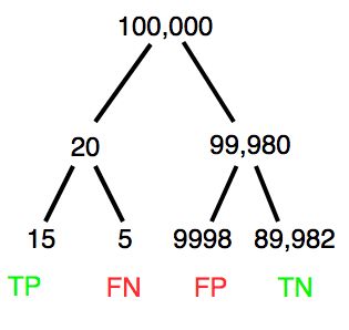
Figure 4. Probability tree for FOBT test; Good test outcomes shown in green: TP stands for true positive and TN stands for true negative. Poor outcomes of a test shown in red: FN stands for false negative and FP stands for false positive.
The associated probabilities for the four possible outcomes of these kinds of tests (e.g., what’s the probability of a person who has tested positive in screening tests actually has the disease?) are shown in Table 1.
Table 1. A 2 X 2 table of possible outcomes of a diagnostic test.
| Person really has the disease | ||
| Test Result | Yes | No |
| Positive | a TP |
b FP |
| Negative | c FN |
d TN |
Bayes’ rule is often given in probabilities,
![\begin{align*} p\left ( D\mid \oplus \right )=\frac{p\left ( D \right )\cdot p\left (\oplus\mid D \right )}{[p\left ( D \right )\cdot p\left (\oplus \right )+p\left ( ND \right )\cdot p\left (\oplus \mid ND \right )]} \end{align*}](https://biostatistics.letgen.org/wp-content/ql-cache/quicklatex.com-fd988801ed9f7a29c963f2df79fcf35c_l3.png "Rendered by QuickLaTeX.com")
Bayes’ rule, where truth is represented by either D (the person really does have the disease”) or ND (the person really does not have the disease”) and ⊕ is symbol for “exclusive or” and reads “not D” in this example.
An easier way to see this is to use frequencies instead. Now, the formula is

Simplified Bayes’ rule, where a is the number of people who test positive and DO HAVE the disease and b is the number of people who test positive and DO NOT have the disease.
Standardized million.
Where did the 100,000 come from? We discussed this in chapter 2: it’s a simple trick to adjust rates to the same population size. We use this to work with natural numbers instead of percent or frequencies. You choose to correct to a standardized population based on the raw incidence rate. A rough rule of thumb:
Table 2. Relationship between standard population size and incidence rate.
| Raw IR rate about | IR | Standard population |
| 1/10 | 10% | 1000 |
| 1/100 | 1% | 10,000 |
| 1/1000 | 0.1% | 100,000 |
| 1/10,000 | 0.01% | 1,000,000 |
| 1/100,000 | 0.001% | 10,000,000 |
| 1/1,000,000 | 0.0001% | 100,000,000 |
The raw incident rate is simply the number of new cases divided by the total population.
Per capita rate.
Yet another standard manipulation is to consider the average incidence per person, or per capita rate. The Latin “per capita” translates to “by head” (Google translate), but in economics, epidemiology, and other fields it is used to reflect rates per person. Tuberculosis is a serious infectious disease of primarily the lungs. Incidence rates of tuberculosis in the United States have trended down since the mid 1900s: 52.6 per 100K in 1953 to 2.7 per 100K in 2019 (CDC). Corresponding per capita values are 5.26 x 10⁻⁴ and 2.7 x 10⁻⁵, respectively. Divide the rate by 100,000 to get per person rate.
Practice and introduce PPV and Youden’s J.
Let’s break these problems down, and in doing so, introduce some terminology common to the field of “risk analysis” as it pertains to biology and epidemiology. Our first example considers the fecal occult blood test, FOBT, test. Blood in the stool may (or may not) indicate polys or colon cancer. (Park et al 2010).
The table shown above will appear again and again throughout the course, but in different forms.
Table 3. A 2 X 2 table of possible outcomes of FOBT test.
| Person really has the disease | |||
| Yes | No | ||
| Positive | 15 | 9998 | PPV = 15/(15+9998) = 0.15% |
| Negative | 5 | 89,982 | NPV = 89982/(89982+5) = 99.99% |
We want to know how good is the test, particularly if the goal is early detection? This is conveyed by the PPV, positive predictive value of the test. Unfortunately, the prevalence of a condition is also at play: the lower the prevalence, the lower the PPV must be, because most positive tests will be false when population prevalence is low.
Youden (1950) proposed a now widely adopted index that summarizes how effective a test is. Youden’s J is the sum of specificity and sensitivity minus one.

where Se stands for sensitivity of the test and Sp stands for sensitivity of the test.
Youden’s J takes on values between 0, for a terrible test, and 1, for a perfect test. For our FOBT example, Youden’s J was 0.65. This statistic looks like it’s independent of prevalence, but it’s use as a decision criterion (e.g., a cutoff value, above which test is positive, below test is considered negative), assumes that the cost of misclassification (false positives, false negatives) are equal. Prevalence affects number of false positives and false negatives for a given diagnostic test, so any decision criterion based on Youden’s J will also be influenced by prevalence (Smits 2010).
Another worked example. A study on cholesterol-lowering drugs (statins) reported a relative risk reduction of death from cardiac event by 22%. This does not mean that for every 1000 people fitting the population studied, 220 people would be spared from having a heart attack. In the study, the death rate per 1000 people was 32 for the statin versus 41 for the placebo — recall that a placebo is a control treatment offered to overcome potential patient psychological bias (see Chapter 5.4). The absolute risk reduction due to statin is only 41 – 32 or 9 in 1000 or 0.9%. By contrast, relative risk reduction is calculated as the ratio of the absolute risk reduction (9) divided by the proportion of patients who died without treatment (41), which is 22% (LIPID Study Group 1998).
Note that risk reduction is often conveyed as a relative rather than as an absolute number. The distinction is important for understanding arguments based in conditional probability. Thus, the question we want to ask about a test is summarized by absolute risk reduction (ARR) and number needed to treat (NNT), and for problems that include control subjects, relative risk reduction (RRR). We expand on these topics in the next section, 7.4 – Epidemiology: Relative risk and absolute risk, explained.
Evidence Based Medicine.
One culture change in medicine is the explicit intent to make decisions based on evidence (Masic et al 2008). Of course, the joke then is, well, what were doctors doing before, diagnosing without evidence? The comic strip xkcd offers one possible answer (Fig 5).
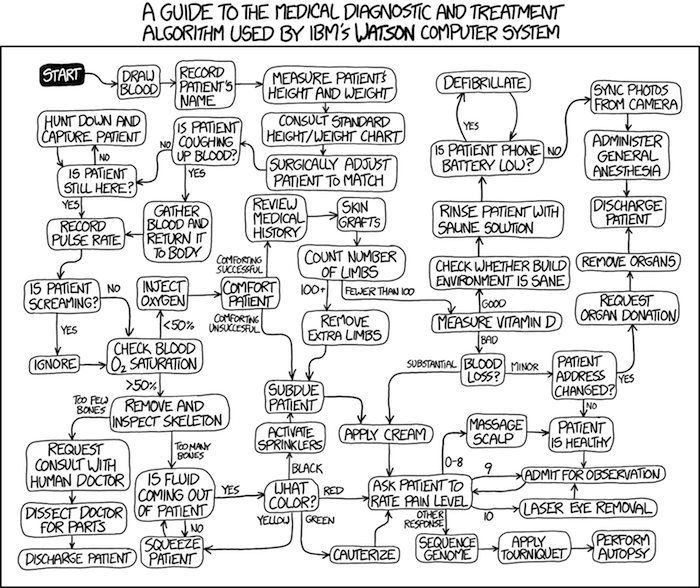
Figure 5. A summary of “evidence based medical” decisions, perhaps? “Watson Medical Algorithm,” https://xkcd.com/1619/.
As you can imagine, there’s considerable reflection about the EBM movement (see discussions in response to Accad and Francis 2018, e.g., Goh 2018). More practically, our objective is for you to be able to work your way through word problems involving risk analysis. You can expect to be asked to calculate, or at least set up for calculation, any of the statistics listed above (e.g., False negative, false positive, etc.). Practice problems are listed at the end of this section, and additional problems are provided to you (Homework 4). You’ll also want to check your work, and in any real analysis, you’d most likely want to use R.
Software.
R has several epidemiology packages, and with some effort, can save you time. Another option is to run your problems in OpenEpi, a browser-based set of tools. OpenEpi is discussed with examples in the next section, 7.4.
Here, we illustrate some capabilities of the epiR package, expanded more also in the next section, 7.4. We’ll use the example from Table 3.
R code
library(epiR)
Table3 <- matrix(c(15, 5, 9998, 89982), nrow = 2, ncol = 2)
epi.tests(Table3)
R output
         Outcome + Outcome -   Total
Test +          15      9998   10013
Test -           5     89982   89987
Total           20     99980  100000

Point estimates and 95% CIs:
--------------------------------------------------------------
Apparent prevalence *                      0.10 (0.10, 0.10)
True prevalence *                          0.00 (0.00, 0.00)
Sensitivity *                              0.75 (0.51, 0.91)
Specificity *                              0.90 (0.90, 0.90)
Positive predictive value *                0.00 (0.00, 0.00)
Negative predictive value *                1.00 (1.00, 1.00)
Positive likelihood ratio                  7.50 (5.82, 9.67)
Negative likelihood ratio                  0.28 (0.13, 0.59)
False T+ proportion for true D- *          0.10 (0.10, 0.10)
False T- proportion for true D+ *          0.25 (0.09, 0.49)
False T+ proportion for T+ *               1.00 (1.00, 1.00)
False T- proportion for T- *               0.00 (0.00, 0.00)
Correctly classified proportion *          0.90 (0.90, 0.90)
--------------------------------------------------------------
* Exact CIs
Oops! I wanted PPV, which by hand calculation was 0.15%, but R reported “0.00?” This is a significant figure reporting issue. The simplest solution is to submit options(digits=6) before the command, then save the output from epi.tests() to an object and use summary(). For example
options(digits=6)
myEpi <- epi.tests(Table3)
summary(myEpi)
And R returns
     statistic           est        lower        upper
1           ap  0.1001300000 0.0982761568  0.102007072
2           tp  0.0002000000 0.0001221693  0.000308867
3           se  0.7500000000 0.5089541283  0.913428531
4           sp  0.9000000000 0.8981238085  0.901852950
5      diag.ac  0.8999700000 0.8980937508  0.901823014
6      diag.or 27.0000000000 9.8110071871 74.304297826
7         nndx  1.5384615385 1.2265702376  2.456532054
8       youden  0.6500000000 0.4070779368  0.815281481
9       pv.pos  0.0014980525 0.0008386834  0.002469608
10      pv.neg  0.9999444364 0.9998703379  0.999981958
11      lr.pos  7.5000000000 5.8193604069  9.666010707
12      lr.neg  0.2777777778 0.1300251423  0.593427490
13      p.rout  0.8998700000 0.8979929278  0.901723843
14       p.rin  0.1001300000 0.0982761568  0.102007072
15      p.tpdn  0.1000000000 0.0981470498  0.101876192
16      p.tndp  0.2500000000 0.0865714691  0.491045872
17      p.dntp  0.9985019475 0.9975303919  0.999161317
18      p.dptn  0.0000555636 0.0000180416  0.000129662
There we go — pv.pos reported as 0.0014980525, which, after turning to a percent and rounding, we have 0.15%. Note also the additional statistics provided — a good rule of thumb — always try to save the output to an object, then view the object, e.g., with summary(). Refer to help pages for additional details of the output (?epi.tests).
What about R Commander menus?
Note 2: Fall 2023 — I have not been able to run the EBM plugin successfully! Simply returns an error message — — on data sets which have in the past performed perfectly. Thus, until further notice, do not use the EBM plugin. Instead, use commands in the epiR package. I’m leaving the text here on the chance the error with the plugin is fixed.
Rcmdr has a plugin that will calculate ARR, RRR and NNT. The plugin is called RcmdrPlugin.EBM (Leucuta et al 2014) and it would be downloaded as for any other package via R.
Download the package from your selected R mirror site, then start R Commander.
install.packages("RcmdrPlugin.EBM")
From within R Commander (Fig 6), select
Tools → Load Rcmdr plug-in(s)…
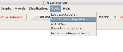
Figure 6. To install an Rcmdr plugin, first go to Rcmdr → Tools → Load Rcmdr plug-in(s)…
Next, select from the list the plug-in you want to load into memory, in this case, RcmdrPlugin.EBM (Fig 7).
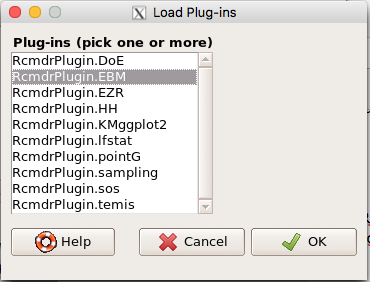
Figure 7. Select the Rcmdr plugin, then click the “OK” button to proceed.
Restart Rcmdr again (Fig 8),
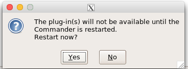
Figure 8. Select “Yes” to restart R Commander and finish installation of the plug-in.
and the menu “EBM” should be visible in the menu bar (Fig 9).
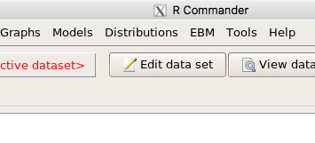
Figure 9. After restart of R Commander the EBM plug-in is now visible in the menu.
Note that you will need to repeat these steps each time you wish to work with a plug-in, unless you modify your .RProfile file. See
Rcmdr → Tools → Save Rcmdr options…
Clicking on the EBM menu item brings up the template for the Evidence Based Medicine module. We’ll mostly work with 2 X 2 tables (e.g., see Table 1) , so select the “Enter two-way table…” option to proceed (Fig 10).
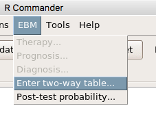
Figure 10. Select “Enter two-way table…”.
And finally, Figure 11 shows the two-way table entry cells along with options. We’ll try a problem by hand then use the EBM plugin to confirm and gain additional insight.
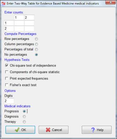
Figure 11. Two-way table Rcmdr EBM plug-in.
For assessing how good a test or assay is, use the Diagnosis option in the EBM plugin. For situations with treated and control groups, use Therapy option. For situations in which you are comparing exposure groups (e.g., smokers vs non-smokers), use the Prognosis option.
Example.
Here’s a simple one (problem from Gigerenzer 2002).
About 0.01% of men in Germany with no known risk factors are currently infected with HIV. If a man from this population actually has the disease, there is a 99.9% chance the tests will be positive. If a man from this population is not infected, there is a 99.9% chance that the test will be negative. What is the chance that a man who tests positive actually has the disease?
Start with the reference, or base population (Figure 12). It’s easy to determine the rate of HIV infection in the population if you use numbers. For 10,000 men in this group, exactly one man is likely to have HIV (0.0001X10,000), whereas 9,999 would not be infected.
For the man who has the disease it’s virtually certain that his results will be positive for the virus (because the sensitivity rate = 99.9%). For the other 9,999 men, one will test positive (the false positive rate = 1 – specificity rate = 0.01%).
Thus, for this population of men, for every two who test positive, one has the disease and one does not, so the probability even given a positive test is only 100*1/2 = 50%. This would also be the test’s Positive Predictive Value.
Note that if the base rate changes, then the final answer changes! For example, if the base rate was 10%
It also helps to draw a tree to help you determine the numbers (Fig 12)
Figure 12. Draw a probability tree to help with the frequencies.
From our probability tree in Figure 12 it is straight-forward to collect the information we need.
- Given this population, how many are expected to have HIV? Two.
- Given the specificity and sensitivity of the assay for HIV, how many persons from this population will test positive? Two.
- For every positive test result, how many men from this population will actually have HIV? One.
Thus, given this population with the known risk associated, the probability that a man testing positive actually has HIV is 50% (=1/(1+1)).
Use the EBM plugin. Select two-way table, then enter the values as shown in Fig 13.
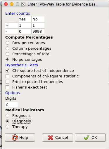
Figure 13. EBM plugin with data entry.
Select the “Diagnosis” option — we are answering the question: How probable is a positive result given information about sensitivity and specificity of a diagnosis test. The results from the EBM functions are given below
Rcmdr> .Table
      Yes No
   +  1    1
   -  0 9998
Rcmdr> fncEBMCrossTab(.table=.Table, .x='', .y='', .ylab='', .xlab='',
Rcmdr+ .percents='none', .chisq='1', .expected='0', .chisqComp='0', .fisher='0',
Rcmdr+ .indicators='dg', .decimals=2)
# Notations for calculations
        Disease + Disease -
Test +      "a"         "b"
Test -      "c"         "d"
# Sensitivity (Se) = 100 (95% CI 2.5 - 100) %. Computed using formula: a / (a + c)
# Specificity (Sp) = 99.99 (95% CI 99.94 - 100) %. Computed using formula: d / (b + d)
# Diagnostic accuracy (% of all correct results) = 99.99 (95% CI 99.94 - 100) %. Computed using formula: (a + d) / (a + b + c + d)
# Youden's index = 1 (95% CI 0.02 - 1). Computed using formula: Se + Sp - 1
# Likelihood ratio of a positive test = 9999 (95% CI 1408.63 - 70976.66). Computed using formula: Se / (Sp - 1)
# Likelihood ratio of a negative test = 0 (95% CI 0 - NaN). Computed using formula: (1 - Se) / Sp
# Positive predictive value = 50 (95% CI 1.26 - 98.74) %. Computed using formula: a / (a + b)
# Negative predictive value = 100 (95% CI 99.96 - 100) %. Computed using formula: d / (c + d)
# Number needed to diagnose = 1 (95% CI 1 - 40.91). Computed using formula: 1 / [Se - (1 - Sp)]
Note that the formulas used to calculate Sensitivity, Specificity, etc., follow our Table 1 (compare to “Notations for calculations”). The use of EBM provides calculations of our confidence intervals.
Questions.
- The sensitivity of the fecal occult blood test (FOBT) is reported to be 0.68. What is the False Negative Rate?
- The specificity of the fecal occult blood test (FOBT) is reported to be 0.98. What is the False Positive Rate?
- For men between 50 and 54 years of age, the rate of colon cancer is 61 per 100,000. If the false negative rate of the fecal occult blood test (FOBT) is 10%, how many persons who have colon cancer will test negative?
- For men between 50 and 54 years of age, the rate of colon cancer is 61 per 100,000. If the false positive rate of the fecal occult blood test (FOBT) is 10%, how many persons who do not have colon cancer will test positive?
- A study was conducted to see if mammograms reduced mortality
Mammogram Deaths/1000 women No 4 Yes 3 data from Table 5-1 p. 60 Gigerenzer (2002)
What is the RRR? - A study was conducted to see if mammograms reduced mortality
Mammogram Deaths/1000 women No 4 Yes 3 data from Table 5-1 p. 60 Gigerenzer (2002)
What is the NNT? - Does supplemental Vitamin C decrease risk of stroke in Type II diabetic women? A study conducted on 1923 women, a total of 57 women had a stroke, 14 in the normal Vitamin C level and 32 in the high Vitamin C level. What is the NNT between normal and high supplemental Vitamin C groups?
- Sensitivity of a test is defined as
A. False Positive Rate
B. True Positive Rate
C. False Negative Rate
D. True Negative Rate - Specificity of a test is defined as
A. False Positive Rate
B. True Positive Rate
C. False Negative Rate
D. True Negative Rate - In thinking about the results of a test of a null hypothesis, Type I error rate is equivalent to
A. False Positive Rate
B. True Positive Rate
C. False Negative Rate
D. True Negative Rate - During the Covid-19 pandemic, number of reported cases each day were published. For example, 155 cases were reported for 9 October 2020 by Department of Health. What is the raw incident rate?
Quiz Chapter 7.3
Conditional Probability and Evidence Based Medicine
Chapter 7 contents
- Introduction
- Epidemiology definitions
- Epidemiology basics
- Conditional Probability and Evidence Based Medicine
- Epidemiology: Relative risk and absolute risk, explained
- Odds ratio
- Confidence intervals
- References and suggested readings