6.5 – Discrete probability distributions
Binomial distribution
Discrete refers to particular outcomes — data that take on only specific separate values. Discrete data types include all of the categorical types we introduced earlier, including binary, ordinal, and nominal.
The binomial probability distribution is a discrete distribution for the number of successes, k, in a sequence of n independent trials, where the outcome of each trial can take on only one of two possible outcomes. For cases of 0 or 1, yes or no, “heads” or “tails,” male or female, pass or fail, we talk about the binomial distribution, because the outcomes are discrete and there can be only two possible (binary) outcomes.
Note 1: The biological definition of sex is binary — whether sexually reproducing organism produces male (sperm) or female (ovum) gametes (cf discussion in Goymann et al 2022). For the argument that sex is a continuum held by some biomedical and social scientists, see Ainsworth 2015.
The mathematical function of the binomial is written as
![\begin{align*} Pr\left [ X \ successes \right ] = \binom{n}{X} p^X \left ( 1-p \right )^{n-X} \end{align*}](https://biostatistics.letgen.org/wp-content/ql-cache/quicklatex.com-3a30d36f8ba1b9fcf3a671be2674d444_l3.png "Rendered by QuickLaTeX.com")
where the binomial coefficient is given by

and X refers to the number of ways to choose “success” from n observations.
Consider an example.
We have to define what we mean by success. For coin toss, this might be the number of heads.
The mean for the binomial this is given simply as

where X is “Heads” (the category of successes for our example), and p corresponds to the probability the selected event occurs, in this case, “Heads.”
The variance of the binomial distribution is given by

Here’s a density plot of two trials with success 2% with n (x) equal to 20 (Fig 1).
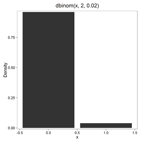
Figure 1. Plot generated with KMggplot2 Rcmdr plugin.
Here’s the R code
Create the trials, 1 through 20, then create an object to hold the number of trials
nSize=1:20
Size <- length(nSize); Size
R returns
[1] 20
Assign the probability value to an object
prob <- 0.02
Next, calculate the mean, mu, and the variance, var, for the binomial with prob = 0.02 and number of trials Size = 20
mu <- Size*prob
var <- Size*prob*(1-prob)
Print the mean and variance; lets assign them to an object then print the object
stats <- c(mu, var); stats
And R returns
[1] 0.400 0.392
And here’s a real-world example. Twinning in humans is rare. In Hawaiʻi in the 1990’s the rate of twin births (monozygotic and dizygotic) was about 20 for every 1000 births or 2%. “Success” here then is twin births.
Figure 2. Example of binomial-like distribution: reported twins born in Hawaiʻi.
Interestingly, rates of twins have since increased in Hawaiʻi (31 out of 1000 births) and in the United States overall (33 out of 1000 births) (Table 2, NCHS Data Brief No. 80, 2012). Data for Fig 2 were for year 2009.
Out of ten births, what is the probability of two twin births in Hawaiʻi?
![\begin{align*} Pr\left [ 2 \ twinbirths \right ] = \left ( \frac{10}{2} \right ) 0.031^2 \left ( 1 - 0.031 \right )^{10-2} \end{align*}](https://biostatistics.letgen.org/wp-content/ql-cache/quicklatex.com-65965fd393d815506757b84eda02c026_l3.png "Rendered by QuickLaTeX.com")
You can solve this with your calculator (yikes!), or take advantage of online calculators (GraphPad QuickCalcs), or use R and Rcmdr.
In R, simply type at the prompt
dbinom(2,10,0.031)
[1] 0.03361446
Try in R Commander.
Rcmdr → Distributions → Discrete distributions → Binomial distribution → Binomial probabilities …

Figure 3. Rcmdr menu to get binomial probability.
Note I used p = 0.033 the rate for entire USA. Here’s the output
> .Table <- data.frame(Pr=dbinom(0:10, size=10, prob=0.033))
> rownames(.Table) <- 0:10
> .Table
Pr
0  7.149320e-01
1  2.439789e-01
2  3.746728e-02 ← Answer, 0.0375 or 3.75%
3  3.409639e-03
4  2.036263e-04
5  8.338782e-06
6  2.371422e-07
7  4.624430e-09
8  5.918028e-11
9  4.487991e-13
10 1.531579e-15
And here is the output for our example from Hawaiʻi (p = 0.031).
> .Table <- data.frame(Pr=dbinom(0:10, size=10, prob=0.031))
> rownames(.Table) <- 0:10
> .Table
Pr
0  7.298570e-01
1  2.334940e-01
2  3.361446e-02 ← Answer, 0.0336 or 3.36%
3  2.867694e-03
4  1.605494e-04
5  6.163507e-06
6  1.643178e-07
7  3.003893e-09
8  3.603741e-11
9  2.561999e-13
10 8.196283e-16
We use the binomial distribution as the foundation for the binomial test, ie, the test of an observed proportion against an expected population level proportion in a Bernoulli trial.
Hypergeometric distribution
The binomial distribution is used for cases of sampling with replacement from a population. When sampling without replacement is done, the hypergeometric distribution is used. It is the number of successes, k, in a sequence of n independent trials drawn from a fixed population.
Note 2: A fixed population in epidemiology refers to a group of individuals, defined by set of characteristics. Examples include individuals selected because they all share a common life event, eg, giving birth. The population is “fixed” because, once an individual is included in the population, they remain a member of the population even if their characteristics change during the duration of the study. The opposite of a fixed population is an dynamic or open population. Definitions from Chapter 2 in Aschengrau and Seage (2003).
This sampling scheme means that each draw is no longer independent — with each draw you decrease the remaining number of observations and thus change the proportion.
The P-value from the hypergeometric distribution is often used to study if genes from a list of Gene Ontology (eg, biological process functional terms like “cell cycle,” or “apoptosis”) are enriched in the sets of genes with expression differences across the treatment groups (cf, discussion in Cao and Zhang 2014). The R package gprofiler2, which links to a Cloud service at g:Profiler, the can be used to do gene enrichment analyses with stunning visualizations (eg, Manhattan plot) suitable for publication.
The mathematical function of the hypergeometric is written as
![\begin{align*} Pr\left [X = k \right ] = \frac{\left ( \frac{K}{k} \right )\left ( \frac{N - K}{n - k} \right )}{\left ( \frac{N}{n} \right )} \end{align*}](https://biostatistics.letgen.org/wp-content/ql-cache/quicklatex.com-4c3fda04d51bcfab12f92b7cd77ff0ad_l3.png "Rendered by QuickLaTeX.com")
where N is the population size, K is the number of successes in that population, and n and k are defined as above. Lets look apply this to the twinning problem.
In 2009, 2200 women gave birth in Hawaiʻi County, Hawaiʻi. Out of 10 births, what is the probability of 2 twin births in Hawaiʻi?
Assuming “risk” of twinning is the same rate as in rest of USA, then we have expected 72 successes in this population (0.033 * 2200).
Here’s the graph (Fig 4).
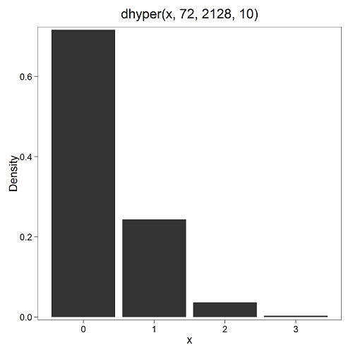
Figure 4. Plot of hypergeometric distribution twinning Hawaiʻi.
where the X axis values shows the number of events with successes (twin births). Taking the bin 2 (we wanted to know about probability of 2 out of ten), we can draw a line back to the Y-axis to get our probability — looks like about 5% roughly. Plot drawn with KMggplot2
To get the actual probability,
Rcmdr → Distributions → Discrete distributions → Hypergeometric distribution → Hypergeometric probabilities …

Figure 5. Rcmdr menu to get hypergeometric probability.
where m is the number of successes, n is the number of “failures,” and k is the number of trials.
> .Table
Pr
0 0.716453457
1 0.243438645
2 0.036688041 ← Answer, 0.0367 or 3.67%
3 0.003228871
The reference to white and black balls and urns is a device described by Bernoulli himself and has been used by others ever since to discuss probability problems (called the urn problem) and so I apply it here to be consistent. The urn contains a number of white (x) and a number of black (y) balls mixed together. One ball is drawn randomly from the urn — what color is it? The ball is then is either returned into the urn (replacement) or it is left out (without replacement) as in the hypergeometric problem, and the selection process is repeated.
Besides applications in gambling and balls-in-urns problems, this distribution is the basis for many tests of gene enrichment from microarray analyses. The hypergeometric forms the basis of the Fisher Exact test (see Chapter 9.5).
Discrete uniform distribution
For discrete cases of “1,” “2,” “3,” “4,” “5,” or “6,” on the single toss of fair dice, we can talk about the discrete uniform distribution because all possible outcomes are equally likely. If you are branded as a “card-counter” in Las Vegas, all you’ve done is reached an understanding of the uniform distribution of card suits!
One biological example would be the fate of a random primary oocyte in the human (mammal) female — three out of four will become polar bodies, eventually reabsorbed, whereas one in four will develop into a secondary oocyte (egg); the uniform distribution has to do with the counts of the products — each of the four primary oocytes has the same (apparently) chance (25%) of becoming the egg (Edwards and Beard 1997).
Analyses in biological research often use a uniform distribution as a baseline or null model (Gotelli and Ulrich 2011). For DNA sequencing, the uniform distribution provides a baseline for assessing coverage bias, eg, GC bias (Ross et al 2013). The uniform distribution underlies the Jukes–Cantor evolutionary model. The Jukes–Cantor model assumes equal substitution rates among all four nucleotides (A, T, C, G) and equal base frequencies (Felsenstein 2003).
The uniform distribution exists also for continuous data types, where every value within a specified interval has equal probability density. For example, DNA shearing during initial library prep for sequencing reactions, breakpoints may be modeled as uniformly distributed along fragment length. Sequence-dependent cleavage bias is concluded when certain DNA fragments or sequences are generated or detected more (or less) frequently than would be expected by chance (Meyer and Liu 2014).
Non-uniform distributions reveal cleavage bias.
Poisson distribution
An extension from the binomial case is that, rather than following success or failure, you may have the following scenario. Consider a wind-dispersed seed released from a plant. If we markup the area around the plant in grids, we could then count the number of seeds within each grid. Most grids will have no seeds, some grids will have one seed, a few grids may have two seeds, etc. Multiple seeds in grids is a rare event. The graph might look like
Figure 6. Example, poisson-like graph: the number of wind-dispersed seeds within each grid.
In molecular biology, use of Poisson distribution is common. In digital PCR for example, a DNA sample is diluted and divided into thousands of small reaction volumes or partitions. Thus, each partition contains either zero molecules, one molecule, or more than one molecule, where the loading of molecules into partitions is assumed to be independent, random, and rare per partition. In sequencing, Poisson models are used to describe random sampling of molecules and reads, especially when coverage is generated by non-deterministic processes like shotgun sequencing.
The Poisson has interesting properties, one being that the expected mean, λ, is equal to the variance. Lambda is, with respect to the Poisson distribution, the average number of times an event happens over a specific period or area.
An equation is
![\begin{align*} Pr\left [X\right ] = \frac{\mu^X e^{-\mu}}{X!} \end{align*}](https://biostatistics.letgen.org/wp-content/ql-cache/quicklatex.com-b172e19511712bb9114f43372f907b6c_l3.png "Rendered by QuickLaTeX.com")
where μ is the mean (or could substitute with variance!), e is the natural logarithm, and X is number of successes you are interested in. For example, if μ = 1, what is the probability of observing a grid with five seeds? Simple enough to do this by hand, but let’s use Rcmdr instead. Here’s the graph (Fig 7) from Rcmdr (KMggplot2 plugin).
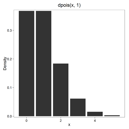
Figure 7. The probability of observing a grid with five seeds, poisson μ = 1 (ggplot2).
and for the actual probability we have from R
dpois(5, lambda = 1)
[1] 0.003065662
Rcmdr → Distributions → Discrete distributions → Poisson distribution → Poisson probabilities … (Fig 8)
The only thing to enter is the mean (some call μ lambda with symbol λ).

Figure 8. Rcmdr menu, poisson probability.
Here’s the output from R. For intervals 0, 1, 2, 3, …, 6 (Rcmdr just enters this range for you!
> .Table <- data.fram(Pr=dpois(0:6, lambda = 1))
> rownames(.Table) <- 0:6
> .Table
Pr
0 0.3678794412
1 0.3678794412
2 0.1839397206
3 0.0613132402
4 0.0153283100
5 0.0030656620 ← Answer, 0.0307 or 3.07%
6 0.0005109437
Next — Continuous distributions
And finally, for ratio (continuous) scale data, which can take on any value, we can express the chance that probability of a given point as a continuous function, with the normal distribution being one of the most important examples (there are others, like the F-distribution). Many statistical procedures assume that the data we use can be viewed as having come from a “normally distributed population.” See Chapter 6.6.
Questions
1.2. Quarterback sacks by game for the NFL team Seahawks, years 2011 through 2022 are summarized below (data extracted from https://www.pro-football-reference.com/ ).
| Sacks | How many games? |
| 0 | 25 |
| 1 | 46 |
| 2 | 49 |
| 3 | 39 |
| 4 | 25 |
| 5 | 14 |
| 6 | 8 |
| 7 | 2 |
| 8 | 1 |
| 9 | 0 |
a) Assuming a Poisson distribution, what are the mean (lambda) and variance?
b) The table covers a total of 112 games. How many sacks (events) were observed?
c) What is the probability of the Seahawks getting zero sacks in a game (in 2022, a season was 17 games; prior years a season was 16 games)?
Quiz Chapter 6.5
Discrete probability
Chapter 6 contents
- Introduction
- Some preliminaries
- Ratios and proportions
- Combinations and permutations
- Types of probability
- Discrete probability distributions
- Continuous distributions
- Normal distribution and the normal deviate
- Moments
- Chi-square distribution
- t distribution
- F distribution
- References and suggested readings