18.4 – Generalized Linear Squares

Introduction
Model variances
Model correlated residuals
Questions
Chapter 18 contents

Introduction

Draft

With access to powerful computers and better algorithms, we can move past the classical ANOVA and ordinary least squares approaches to linear models. We have discussed general linear models, but here we introduce generalized linear models, GLM. What follows is just a brief foray; for more — and better! discussion, see Zuur et al (2009).

Model variances

Data from Corn and Hiesey (1973) ohia.RData

> head(ohia)
   Site  Height   Width
1   M-1 12.5567 19.1264
2   M-1 13.2019 13.1547
3   M-1  8.0699 16.0320
4   M-1  6.0952 22.8586
5   M-1 11.3879 11.0105
6   M-1 12.2242 21.8102

# ignore the variance issue

> AnovaModel.1 <- aov(Height ~ Site, data = ohia); summary(AnovaModel.1)
           Df Sum Sq Mean Sq F value      Pr(>F) 
Site        2   4070  2034.8   22.63 0.000000131 ***
Residuals  47   4227    89.9 
---
Signif. codes: 0 '***' 0.001 '**' 0.01 '*' 0.05 '.' 0.1 ' ' 1

Alternatively, use gls(). Default fits by restricted maximum likelihood, REML. That is, it’s the likelihood of linear combinations of the original data.

>model.aov.1 <- gls(Height ~ Site, data = ohia)

Generalized least squares fit by REML
Model: Height ~ Site 
Data: ohia 
     AIC      BIC    logLik
361.1312 368.5318 -176.5656

Coefficients:
                Value Std.Error  t-value p-value
(Intercept) 15.313745  2.120550 7.221591  0.0000
Site[T.M-2] 19.261000  2.998911 6.422666  0.0000
Site[T.M-3]  2.924215  3.672900 0.796160  0.4299

Correlation: 
            (Intr) S[T.M-2
Site[T.M-2] -0.707 
Site[T.M-3] -0.577 0.408

Standardized residuals:
       Min         Q1        Med        Q3       Max 
-1.9832938 -0.5020880 -0.1850871 0.5017636 3.0850635

Residual standard error: 9.483388 
Degrees of freedom: 50 total; 47 residual

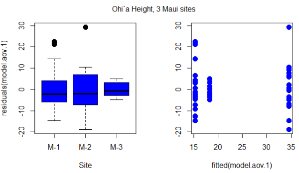
Left: Box plot residuals from simple one-way ANOVA vs predictors (sites). Right: residuals from simple one-way ANOVA vs predictors (sites)

Figure 1. Box plot of residuals from GLS model by elevation site predictors (left) and scatterplot of residuals by fitted values from GLS model (right).

Code for the plot in Figure 1

par(mfrow = c(1, 2))
plot(residuals(model.aov.1) ~ Site, pch=19, cex=1.5,col=”blue”, data = ohia)
plot(residuals(model.aov.1) ~ fitted(model.aov.1), pch=19, cex=1.5, col=”blue”, ylab=””, data=ohia)
mtext(“ANOVA Ohi`a Height, 3 Maui sites “, side = 3, line = -3, outer = TRUE)

# test equal variances, Height

> leveneTest(Height ~ Site, data=ohia, center="median")
Levene's Test for Homogeneity of Variance (center = "median")
      Df F value  Pr(>F)
group  2  2.1663  0.1259
      47

We would conclude no significant departures from equal variances.

> bartlett.test(Height ~ Site, data=ohia)

Bartlett test of homogeneity of variances

data:  Height by Site
Bartlett's K-squared = 10.373, df = 2, p-value = 0.005592

Bartlett’s sensitive to deviations from normality

Include variances as part of model

> model.aov.3 <- gls(Height ~ Site, data = ohia, weights = varIdent(form = ~1|Site)); summary(model.aov.3)
Generalized least squares fit by REML
Model: Height ~ Site
Data: ohia
    AIC      BIC    logLik
354.421 365.5219 -171.2105

varIdent permits variances for each group to vary. Results from R continue below.

Variance function:
 Structure: Different standard deviations per stratum
 Formula: ~1 | Site
 Parameter estimates:
      M-1       M-2       M-3
1.0000000 1.0396880 0.3471771

We see here that comparisons were carried out versus M-1 site.

Coefficients:
                Value Std.Error  t-value p-value
(Intercept) 15.313745  2.280931 6.713812  0.0000
Site[T.M-2] 19.261000  3.290358 5.853770  0.0000
Site[T.M-3]  2.924215  2.541027 1.150800  0.2556

Marginal differences between M-1 and M-2 for height were significantly different, but not between M-1 and M-3 site.

Correlation:
            (Intr) S[T.M-2
Site[T.M-2] -0.693
Site[T.M-3] -0.898 0.622

Standardized residuals:
       Min         Q1        Med        Q3       Max
-1.7734556 -0.6909962 -0.2108834 0.5801370 2.7586550

Residual standard error: 10.20064
Degrees of freedom: 50 total; 47 residual

# Test the models

> anova(model.aov.1, model.aov.3)
            Model df      AIC      BIC    logLik   Test  L.Ratio p-value
model.aov.1     1  4 361.1312 368.5318 -176.5656 
model.aov.3     2  6 354.4210 365.5219 -171.2105 1 vs 2  10.7102 0.0047

Although additional degrees of freedom are required, note that this model (model.aov.3) has higher (better!) log likelihood (-171.21) than model.aov.1, the gls model lacking a fit for different variances (-176.57). Introduce a test of the hypothesis that the two models are equal by comparing the log (natural) likelihoods, the log likelihood ratio test, LRT.

$\begin{align*} LRT=-2\cdot ln\left ( \frac{LL\ model \1}{LL \ model \2} \right ) = -2\cdot ln \left [ \left (LL\ model \1 \right ) - \left (LL \ model \2 \right ) \right ] \end{align*}$

The LRT follows a chi-square distribution (per Wilk’s theorem). If there was no advantage to fitting for unequal variances, then the model fit would not be improved and p-value of the LRT would not be less than 5%.

Conclusion

You can see why this approach, modeling versus separate test of assumptions would be the preferred way to go. We get a better fitting model, cf discussion in

Another example, same data set.

# ignore variances, Width
model.aov.2 <- gls(Width ~ Site, data = ohia); summary(model.aov.2)

Figure 2.

par(mfrow = c(1, 2))
plot(residuals(model.aov.2) ~ Site, pch=19, cex=1.5,col=”blue”, data = ohia)
plot(residuals(model.aov.2) ~ fitted(model.aov.2), pch=19, cex=1.5, col=”blue”, ylab=””, data=ohia)
mtext(“ANOVA Ohi`a Width 3 Maui sites “, side = 3, line = -3, outer = TRUE)

# test equal variances, Width
Tapply(Width ~ Site, var, na.action=na.omit, data=ohia) # variances by group
leveneTest(Width ~ Site, data=ohia, center=”median”)
Tapply(Width ~ Site, var, na.action=na.omit, data=ohia) # variances by group
bartlett.test(Width ~ Site, data=ohia)

# model the variances, Height

library(nlme)
model.aov.3 <- gls(Height ~ Site, data = ohia, weights = varIdent(form = ~1|Site)); summary(model.aov.3)
par(mfrow = c(1, 2))
plot(residuals(model.aov.3) ~ Site, pch=19, cex=1.5,col=”red”, data = ohia)
plot(residuals(model.aov.3) ~ fitted(model.aov.3), pch=19, cex=1.5, col=”red”, ylab=””, data=ohia)
mtext(“GLS Ohi`a Height 3 Maui sites “, side = 3, line = -3, outer = TRUE)

# Test the models
anova(model.aov.1, model.aov.3)

# model the variances, Width
model.aov.4 <- gls(Width ~ Site, data = ohia, weights = varIdent(form = ~1|Site)); summary(model.aov.4)
par(mfrow = c(1, 2))
plot(residuals(model.aov.4) ~ Site, pch=19, cex=1.5,col=”red”, data = ohia)
plot(residuals(model.aov.4) ~ fitted(model.aov.4), pch=19, cex=1.5, col=”red”, ylab=””, data=ohia)
mtext(“GLS Ohi`a Width 3 Maui sites “, side = 3, line = -3, outer = TRUE)

# Test the models
anova(model.aov.2, model.aov.4)

Model correlated residuals

[pending]

Questions

[pending]

Chapter 18 contents

Introduction
Multiple linear regression
Nonlinear regression
Logistic regression
Generalized Linear Squares
Selecting the best model
Compare two linear models
References and suggested readings (Ch17 & 18)