5.5 – Importance of randomization in experimental design
Introduction
If the goal of the research is to make general, evidenced-based statements about causes of disease or other conditions of concern to the researcher, then how the subjects are selected for study directly impacts our ability to make generalizable conclusions. The most important concept to learn about inference in statistical science is that your sample of subjects upon which all measurements and treatments are conducted, ideally should be a random selection of individuals from a well-defined reference population.
The primary benefit of random sampling is that it strengthens our confidence in the links between cause and effect. Often after an intervention trial is complete, differences among the treatment groups will be observed. Groups of subjects who participated in sixteen weeks of “vigorous” aerobic exercise training show reduced systolic blood pressure compared to those subjects who engaged in light exercise for the same period of time (Cox et al 1996). But how do we know that exercise training caused the difference in blood pressure between the two treatment groups? Couldn’t the differences be explained by chance differences in the subjects? Age, body mass index (BMI), overall health, family history, etc?
How can we account for these additional differences among the subjects? If you are thinking like an experimental biologist, then the word “control” is likely coming to the foreground. Why not design a study in which all 60 subjects are the same age, the same BMI, the same general health, the same family … history…? Hmm. That does not work. Even if you decide to control age, BMI, and general health categories, you can imagine the increased effort and cost to the project in trying to recruit subjects based on such narrow criteria. So, control per se is not the general answer.
If done properly, random sampling makes these alternative explanations less likely. Random sampling implies that other factors that may causally contribute to differences in the measured outcome, but themselves are not measured or included as a focus of the research study, should be the same, on average, among our different treatment groups. The practical benefits of proper random sampling is that recruiting subjects gets easier — fewer subjects will be needed because you are not trying to control dozens of factors that may (or may not!) contribute to differences in your outcome variable. The downside to random sampling is that the variability of the outcomes within your treatment groups will tends to increase. As we will see when we get to statistical inference, large variability within groups will make it less likely that any statistical difference between the treatment groups will be observed.
Demonstrate the benefits of random sampling as a method to control for extraneous factors.
The study reported by Cox et al included 60 obese men between the ages of 20 and 50. A reasonable experimental design decision would suggest that the 60 subjects be split into the two treatment groups such that both groups had 30 subjects for a balanced design. Subjects who met all of the research criteria and who had signed the informed consent agreement are to be placed into the treatment groups and there are many ways that group assignment could be accomplished. One possibility, the researchers could assign the first 30 people that came into the lab to the Vigorous exercise group and the remaining 30 then would be assigned to the Light exercise group. Intuitively I think we would all agree that this is a suspect way to design an experiment, but more importantly, why shouldn’t you use this convenient method?
Just for argument’s sake, imagine that their subjects came in one at a time, and, coincidentally, they did so by age. The first person was age 21, the second was 22, and so on up to the 30th person who was 50. Then, the next group came in, again, coincidentally in order of ascending age. If you calculate the simple average age for each group you will find that they are identical (35.5 years). On the surface, this looks like we have controlled for age: both treatment groups have subjects that are the same age. A second option is to sort the subjects into the two treatment groups so that a 21 year old is in Group A, and the other 21 year old is in Group B, and so on. Again, the average age of Group A subjects and of Group B subjects would be the same and therefore controlled with respect to any covariation between age and change in blood pressure. However, there are other variables that may covary with blood pressure, and by controlling one, we would need to control the others. Randomization provides a better way.
I will demonstrate how randomization tends to distribute the values in such a way that the groups will not differ appreciably for the nuisance variables like age and BMI differences and, by extension, any other covariable. The R work is attached following the Reading list. The take-home message: After randomly selecting subjects for assignment to the treatment groups, the apparent differences between Group A and Group B for both age and BMI are substantially diminished. No attempt to match by age and by BMI is necessary. The numbers are shown in the table and then in two graphics (Fig. 1, Fig. 2) derived from the table.
Table 1. Mean age and BMI for subjects in two treatment groups A and B where subjects were assigned randomly or by convenience to treatment groups.
| Group | Random assignment of subjects to treatment groups | Convenience assignment of subjects to treatment groups |
|---|---|---|
| A | 35.2 | 28 |
| B | 35.8 | 43 |
| A | 32.49 | 28.99 |
| B | 32.87 | 37.37 |
Just for emphasis, the means from Table 1 are presented in the next two figures (Fig 1 and Fig 2).
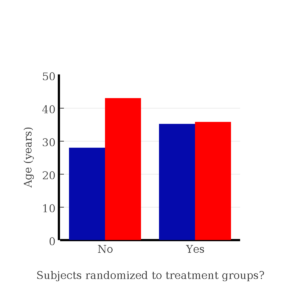
Figure 1. Age of subjects by groups (A = blue, B = red) with and without randomized assignment of subjects to treatment groups
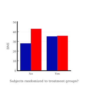
Figure 2. BMI of subjects by groups (A = blue, B = red) with and without randomized assignment of subjects to treatment groups
Note that the apparent difference between A and B for BMI disappear once proper randomization of subjects was accomplished. In conclusion, a random sample is an approach to experimental design that helps to reduce the influence other factors may have on the outcome variable (e.g., change in blood pressure after 16 weeks of exercise). In principle, randomization should protect a project because, on average, these influences will be represented randomly for the two groups of individuals. This reasoning extends to unmeasured and unknown causal factors as well.
This discussion was illustrated by random assignment of subjects to treatment groups. The same logic applies to how to select subjects from a population. If the sampling is large enough, then a random sample of subjects will tend to be representative of the variability of the outcome variable for the population and representative also of the additional and unmeasured cofactors that may contribute to the variability of the outcome variable.
What about observational studies? How does randomization work?
However, if you do cannot obtain a random sample, then conclusions reached may be sample-specific, biased. …perhaps the group of individuals that likes to exercise on treadmills just happens to have a higher cardiac output because they are larger than the individuals that like to exercise on bicycles. This nonrandom sample will bias your results and can lead to incorrect interpretation of results. Random sampling is CRUCIAL in epidemiology, opinion survey work, most aspects of health, drug studies, medical work with human subjects. It’s difficult and very costly to do… so most surveys you hear about, especially polls reported from Internet sites, are NOT conducted using random sampling (included in the catch-all term “probability sampling“)!! As an aside, most opinion survey work involves complex sample designs involving some form of geographic clustering (e.g., all phone numbers in a city, random sample among neighborhoods).
Random sampling is the ideal if generalizations are to be made about data, but strictly random sampling is not appropriate for all kinds of studies. Consider the question of whether or not EMF exposure is a risk factor for developing cancer (Pool 1990). These kinds of studies are observational: at least in principle, we wouldn’t expect that housing and therefore exposure to EMF is manipulated (cf. discussion Walker 2009). Thus, epidemiologists will look for patterns: if EMF exposure is linked to cancer, then more cases of cancer should occur near EMF sources compared to areas distant from EMF sources. Thus, the hypothesis is that an association between EMF exposure and cancer occurs non-randomly, whereas cancers occurring in people not exposed to EMF are random. Unfortunately, clusters can occur even if the process that generates the data is random.
Compare Graph A and Graph B (Fig 3). One of the graphs resulted from a random process and the other was generated by a non-random process. Note that the claim can be rephrased about the probability that each grid has a point, eg, it’s like Heads/Tails of 16 tosses of a coin. We can see clusters of points in Graph B; Graph A lacks obvious clusters of points — there is a point in each of the 16 cells of the grid. Although both patterns could be random, the correct answer in this case is Graph B.
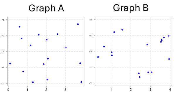
Figure 3. An example of clustering resulting from a random sampling process (Graph B). In contrast, Graph A was generated so that a point was located within each grid.
Hard to tell — and truth be told, random process could generate either one. To convince you, Figure 4 reveals the grouping that was done for Group A, in contrast with Group B which was drawn with the truly random process.
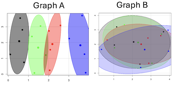
Figure 4. Same graphs as Figure 3, but with ellipses around the grouped data (hard to tell, but the centroids are the larger points).
Implications for sampling
The graphic below shows the transmission grid in the continental United States (Fig 5). How would one design a random sampling scheme overlaid against the obviously heterogeneous distribution of the grid itself? If a random sample was drawn, chances are good that no population would be near a grid in many of the western states, but in contrast, the likelihood would increase in the eastern portion of the United States where the population and therefore transmission grid is more densely placed.
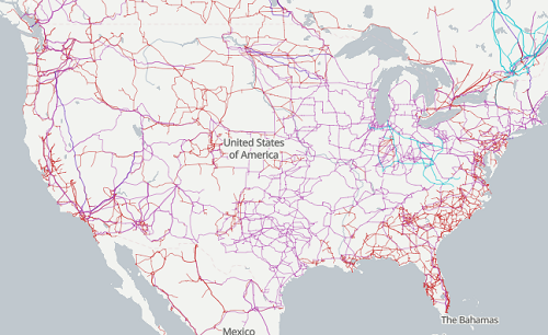
Figure 5. Map of electrical transmission grid for continental United States of America. Image source https://openinframap.org/#3/24.61/-101.16
For example, you want to test whether or not EMF affects human health, and your particular interest is in whether or not there exists a relationship between living close to high voltage towers or transfer stations and brain cancer. How does one design a study, keeping in mind the importance of randomization for our ability to generalize and assign causation? This is a part of epidemiology which strives to detect whether clusters of disease are related to some environmental source. It is an extremely difficult challenge. For the record, no clear link to EMF and cancer has been found, but reports do appear from time to time (e.g., report on a cluster of breast cancer in men working in office adjacent to high EMF, Milham 2004).
Questions
1. Use the sample() with and without replacement on the object (see help with R below)
fruit <- c("apple", "banana", "grape", "kiwi", "pear", "pineapple", "tomato")a) set of 3
b) set of 4
2. Confirm the claim by calculating the probability of Graph A result vs Graph B result (see R script below).
Quiz Chapter 5.5
Importance of randomization in experimental design
R code!
Code you type is shown in red; responses or output from R are shown in blue. Recall that statements preceded by the hash # are comments and are not read by R (i.e., no need for you to type them).
First, create some variables. Vectors aa and bb contain my two age sequences.
 aa = seq(21,50)
 bb = seq(21,50)
Second, append vector bb to the end of vector aa
 age = append(aa,bb)
 age           #submit the vector (variable) name to print the records for verification - looks good!
  [1] 21 22 23 24 25 26 27 28 29 30 31 32 33 34 35 36 37 38 39 40 41 42 43 44 45 46 47 48 49 50 21 22 23 24 25 26 27 28 29 30 31 32 33 34 35 36 37
 [48] 38 39 40 41 42 43 44 45 46 47 48 49 50
Third, get the average age for the first group (the aa sequence) and for the second group (the bb sequence). Lots of ways to do this, I made a two subsets from the combined age variable; could have just as easily taken the mean of aa and the mean of bb (same thing!).
 A = age[1:30]
 mean(A)
 [1] 35.5
 B = age[31:60]
 mean(B)
 [1] 35.5
Fourth, start building a data frame, then sort it by age. Will be adding additional variables to this data frame
 ex.random = data.frame(age)
 AO.all = sort(ex.random$age)
 AO.age           #submit the vector (variable) name to print the records for verification - looks good!
  [1] 21 21 22 22 23 23 24 24 25 25 26 26 27 27 28 28 29 29 30 30 31 31 32 32 33 33 34 34 35 35 36 36 37 37 38 38 39 39 40 40 41 41 42 42 43 43 44
 [48] 44 45 45 46 46 47 47 48 48 49 49 50 50
Fifth, divide the variable again into two subsets of 30 and get the averages
 AO = AO.age[1:30]
 AO
  [1] 21 21 22 22 23 23 24 24 25 25 26 26 27 27 28 28 29 29 30 30 31 31 32 32 33 33 34 34 35 35
 mean(AO)
 [1] 28
 BO = AO.age[31:60]
 BO
  [1] 36 36 37 37 38 38 39 39 40 40 41 41 42 42 43 43 44 44 45 45 46 46 47 47 48 48 49 49 50 50
 mean(BO)
 [1] 43
Sixth, create an index variable, random order without replacement
rand.index = sample(1:60,60,replace=F)Add the new variable to our existing data frame, then print it to check that all is well
 ex.random$rand = rand.index
 ex.random
    age rand
 1   21   43
 2   22   15
 3   23   17
 4   24   35
 5   25   19
 6   26   18
 7   27   22
 8   28   31
 9   29   12
 10  30   44
 11  31   24
 12  32    5
 13  33    2
 14  34   50
 15  35   23
 16  36   20
 17  37   41
 18  38   56
 19  39   36
 20  40    8
 21  41   45
 22  42   38
 23  43   42
 24  44   46
 25  45   16
 26  46   21
 27  47   28
 28  48   10
 29  49   32
 30  50   54
 31  21   57
 32  22   51
 33  23   27
 34  24   40
 35  25   14
 36  26   48
 37  27   26
 38  28   58
 39  29    9
 40  30   11
 41  31    4
 42  32   52
 43  33   37
 44  34   53
 45  35    6
 46  36   34
 47  37   39
 48  38    7
 49  39    1
 50  40   47
 51  41   33
 52  42   60
 53  43   49
 54  44   30
 55  45   29
 56  46   55
 57  47   13
 58  48    3
 59  49   25
 60  50   59
Seventh, select for our first treatment group the first 30 subjects from the randomized index. There are again other ways to do this, but sorting on the index variable means that the subject order will be change too.
AR.age = ex.random[order(ex.random$rand),] #created a new data frame to distinguish it from the presorted version "ex.random"Print the new data frame to confirm that the sorting worked. It did. we can see that the rows have been sorted by ascending order based on the index variable.
 AR.age
    age rand
 49  39    1
 13  33    2
 58  48    3
 41  31    4
 12  32    5
 45  35    6
 48  38    7
 20  40    8
 39  29    9
 28  48   10
 40  30   11
 9   29   12
 57  47   13
 35  25   14
 2   22   15
 25  45   16
 3   23   17
 6   26   18
 5   25   19
 16  36   20
 26  46   21
 7   27   22
 15  35   23
 11  31   24
 59  49   25
 37  27   26
 33  23   27
 27  47   28
 55  45   29
 54  44   30
 8   28   31
 29  49   32
 51  41   33
 46  36   34
 4   24   35
 19  39   36
 43  33   37
 22  42   38
 47  37   39
 34  24   40
 17  37   41
 23  43   42
 1   21   43
 10  30   44
 21  41   45
 24  44   46
 50  40   47
 36  26   48
 53  43   49
 14  34   50
 32  22   51
 42  32   52
 44  34   53
 30  50   54
 56  46   55
 18  38   56
 31  21   57
 38  28   58
 60  50   59
 52  42   60
Eighth, create our new treatment groups, again of n = 30 each, then get the means ages for each group.
 AR = AR.age$age[1:30]
 mean(AR)
 [1] 35.16667
 AR2 = AR.all$all[31:60]
 mean(AR2)
 [1] 35.83333
Get the minimum and maximum values for the groups
 min(AR)
 [1] 22
 min(AR2)
 [1] 21
 max(AR)
 [1] 49
 max(AR2)
 [1] 50
Ninth, create a BMI variable drawn from a normal distribution with coefficient of variation equal to 20%. The first group with we will call cc
cc = rnorm(n=30,m=27.5, sd=5.5) #mean was 27.5 for this group with standard deviation of 5.5The second group called dd
dd = rnorm(n=30,m=37.5, sd=7.5) #mean was 37.5 for this group with standard deviation of 7.5Create a new variable called BMI by joining cc and dd
 BMI=append(cc,dd)
 BMI            #print out BMI to confirm. Looks good!
  [1] 27.87528 27.83250 31.88703 34.99041 24.06751 23.50952 22.57779 31.48394 31.04321 25.60258 25.41081 22.34619 34.62213 36.41348 41.17740
 [16] 20.56529 27.25238 21.85205 32.11690 32.37168 23.11314 33.29110 34.99106 38.22016 18.72105 26.22030 25.13412 27.50475 34.79361 32.81267
 [31] 47.57872 27.58428 40.17211 38.22195 26.91893 37.02784 53.72671 34.94727 30.35245 38.32571 40.52111 36.15627 30.36592 36.20397 47.63142
 [46] 40.30846 36.47643 50.86804 43.63741 37.84994 42.82665 41.71008 28.44976 24.57906 42.37762 38.38512 35.22879 31.34063 34.02996 27.28038
Add the BMI variable to our data frame.
 ex.random$BMI = BMI
 ex.random              #Print out the revised data frame. Looks good. We now have three variables: age, the index "rand," and now BMI
    age rand      BMI
 1   21   43 27.87528
 2   22   15 27.83250
 3   23   17 31.88703
 4   24   35 34.99041
 5   25   19 24.06751
 6   26   18 23.50952
 7   27   22 22.57779
 8   28   31 31.48394
 9   29   12 31.04321
 10  30   44 25.60258
 11  31   24 25.41081
 12  32    5 22.34619
 13  33    2 34.62213
 14  34   50 36.41348
 15  35   23 41.17740
 16  36   20 20.56529
 17  37   41 27.25238
 18  38   56 21.85205
 19  39   36 32.11690
 20  40    8 32.37168
 21  41   45 23.11314
 22  42   38 33.29110
 23  43   42 34.99106
 24  44   46 38.22016
 25  45   16 18.72105
 26  46   21 26.22030
 27  47   28 25.13412
 28  48   10 27.50475
 29  49   32 34.79361
 30  50   54 32.81267
 31  21   57 47.57872
 32  22   51 27.58428
 33  23   27 40.17211
 34  24   40 38.22195
 35  25   14 26.91893
 36  26   48 37.02784
 37  27   26 53.72671
 38  28   58 34.94727
 39  29    9 30.35245
 40  30   11 38.32571
 41  31    4 40.52111
 42  32   52 36.15627
 43  33   37 30.36592
 44  34   53 36.20397
 45  35    6 47.63142
 46  36   34 40.30846
 47  37   39 36.47643
 48  38    7 50.86804
 49  39    1 43.63741
 50  40   47 37.84994
 51  41   33 42.82665
 52  42   60 41.71008
 53  43   49 28.44976
 54  44   30 24.57906
 55  45   29 42.37762
 56  46   55 38.38512
 57  47   13 35.22879
 58  48    3 31.34063
 59  49   25 34.02996
 60  50   59 27.28038
Tenth, repeat our protocol from before: Set up two groups each with 30 subjects, calculate the means for the variables and then sort by the random index and get the new group means.
 AO = ex.random$BMI[1:30]
 mean(AO)
 [1] 28.99333
 BO = ex.random$BMI[31:60]
 mean(BO)
 [1] 37.36943
All we did was confirm that the unsorted groups had mean BMI of around 27.5 and 37.5 respectively. Now, proceed to sort by the random index variable. Go ahead and create a new data frame
 AR.age = ex.random[order(ex.random$rand),]
 AR.age                 #Print out the new data frame to confirm. Looks good.
    age rand      BMI
 49  39    1 43.63741
 13  33    2 34.62213
 58  48    3 31.34063
 41  31    4 40.52111
 12  32    5 22.34619
 45  35    6 47.63142
 48  38    7 50.86804
 20  40    8 32.37168
 39  29    9 30.35245
 28  48   10 27.50475
 40  30   11 38.32571
 9   29   12 31.04321
 57  47   13 35.22879
 35  25   14 26.91893
 2   22   15 27.83250
 25  45   16 18.72105
 3   23   17 31.88703
 6   26   18 23.50952
 5   25   19 24.06751
 16  36   20 20.56529
 26  46   21 26.22030
 7   27   22 22.57779
 15  35   23 41.17740
 11  31   24 25.41081
 59  49   25 34.02996
 37  27   26 53.72671
 33  23   27 40.17211
 27  47   28 25.13412
 55  45   29 42.37762
 54  44   30 24.57906
 8   28   31 31.48394
 29  49   32 34.79361
 51  41   33 42.82665
 46  36   34 40.30846
 4   24   35 34.99041
 19  39   36 32.11690
 43  33   37 30.36592
 22  42   38 33.29110
 47  37   39 36.47643
 34  24   40 38.22195
 17  37   41 27.25238
 23  43   42 34.99106
 1   21   43 27.87528
 10  30   44 25.60258
 21  41   45 23.11314
 24  44   46 38.22016
 50  40   47 37.84994
 36  26   48 37.02784
 53  43   49 28.44976
 14  34   50 36.41348
 32  22   51 27.58428
 42  32   52 36.15627
 44  34   53 36.20397
 30  50   54 32.81267
 56  46   55 38.38512
 18  38   56 21.85205
 31  21   57 47.57872
 38  28   58 34.94727
 60  50   59 27.28038
 52  42   60 41.71008
Get the means of the new groups
 AR = AR.age$BMI[1:30]
 mean(AR)
 [1] 32.49004
 min(AR)
 [1] 18.72105
 max(AR)
 [1] 53.72671
 AR2 = AR.all$BMI[31:60]
 mean(AR2)
 [1] 33.87273
 min(AR2)
 [1] 21.85205
 max(AR2)
 [1] 47.57872
That’s all of the work!
Data set
nonrandom
| X | Y |
| 0.779 | 0.747 |
| 0.098 | 1.248 |
| 0.697 | 2.811 |
| 0.59 | 3.553 |
| 1.295 | 0.075 |
| 1.858 | 1.207 |
| 1.172 | 2.388 |
| 1.597 | 3.051 |
| 2.051 | 0.242 |
| 2.081 | 1.546 |
| 2.016 | 2.738 |
| 2.587 | 3.088 |
| 3.833 | 0.088 |
| 3.776 | 1.264 |
| 3.017 | 2.254 |
| 3.657 | 3.712 |
random
| X1 | Y1 |
| 1.157 | 3.203 |
| 2.407 | 0.62 |
| 1.033 | 1.946 |
| 3.676 | 2.866 |
| 3.57 | 2.703 |
| 3.056 | 0.685 |
| 1.568 | 3.355 |
| 1.041 | 1.753 |
| 0.643 | 2.295 |
| 2.884 | 0.687 |
| 3.53 | 2.591 |
| 2.838 | 2.431 |
| 3.945 | 1.518 |
| 0.34 | 1.64 |
| 2.45 | 0.386 |
| 3.921 | 2.976 |
Chapter 5 contents
- The basics explained
- Experiments
- Experimental and Sampling units
- Replication, Bias, and Nuisance Variables
- Clinical trials
- Importance of randomization in experimental design
- Sampling from Populations
- References and suggested readings