3.2 – Measures of Central Tendency
- Introduction to summary statistics.
- Other “means”.
- How to calculate these other means.
- Do try on your own!.
- Other measures of central tendency.
- Why the median may be a better middle than the mean.
- Scaling and transformation of data.
- R operators.
- Creating objects in R.
- R code calculate central tendency.
- There’s an R package for that.
- Use aggregate() to calculate summary statistics by group.
- Questions.
- Quiz.
- Chapter 3 contents .
Introduction to summary statistics.
For a sample of observations we can begin the summary by identifying the “typical” value. Various statistics are used to describe the middle and collectively these are referred to as measures of central tendency. The mean, the median, and the mode are the most common measures of central tendency. In the situation in which we work with data from a population census, we would calculate population descriptive statistics — not inferential statistics; because we more often work with samples from populations, we report sample descriptive statistics.
First we review the familiar arithmetic mean and introduce the weighted mean. Next we introduce “other means,” which you may not be as familiar with.
Means.
There are several means beyond the simple arithmetic average or mean. Here we review a few. We use this topic also to start introducing standard notation we will use throughout the book.
The population mean, μ (pronounced “mu”) is given by
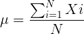
Xi, an observation on the i-th individual
Σ, or “sigma,” which instructs you to add them up (the X’s), from i = 1 (the first observation) to i = N (the last observation).
The sample mean,  , pronounced “eks bar,” of a collection of observations is given by
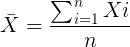
Note 1: Parameters (aka random variables) get Greek letters and sample variables get Roman letters. See Chapter 3.4
Weighted arithmetic mean.
In some cases you may have several samples from the same population. If the sample sizes are the same, you can calculate the average of averages without any fuss — just take all of the sample means and add them up, then divide by the total number of samples. If the sample sizes differ, then you needs to weight (W) each sample mean by its sample size. Simply divide each sample mean by its appropriate sample size, then add all of these up. That is the weighted average.
More generally, we can write

For example, consider a variable containing the following observations, for example, over the course of watching birds gathering at a drinking source (eg, recorded over 20 days, a single 5 minute interval per day), we can count how many times zero, one, two, etc birds are observed.
Table 1. A sample of counts of observations, eg, how many birds
| Observation | Frequency |
|---|---|
| 1 | 0 |
| 2 | 0 |
| 3 | 2 |
| 4 | 4 |
| 5 | 2 |
| 6 | 3 |
| 7 | 2 |
| 8 | 3 |
| 9 | 1 |
The observation “4” was observed four times; the observation “5” was observed twice, and so on for a total of 15 observations.
What is the arithmetic mean of these 15 observations? To solve this, well, you have a couple of choices. You could copy the numbers down as often as they appear and then calculate the mean in the usual way.
Other “means”.
The arithmetic average (illustrated above) is not the only way to estimate the mean.
The trimmed mean, also called the truncated mean, is a useful approach when data is widely dispersed — data spread away from the middle (see Chapter 3.3). Thus, the trimmed mean will be less influenced compared to the arithmetic mean by outlier data points, ie, data far from other data points in the set.
You would use the trimmed mean to describe the middle of a data set in which a plot shows most of the values are clumped together around a middle – and yet you see a few values that are much smaller or much greater. A specified percentage of the smallest and largest values are removed from the data set and then the simple arithmetic mean is calculated for the trimmed data set. For example, given a data set of daily rainfall for different cities, you might wish to remove the driest 5% and wettest 5% of the days in order to better compare the rainfall trends for the cities.
Calculating the trimmed mean is straight-forward in R: use the same built-in function, mean(), but add some options.
Note 2: This is a good time to remind you how to get help with R commands. Do you recall how to get help in R?
At the R prompt type
help(mean) or
?mean
The R Documentation page for mean() will pop up (assuming you allowed R to install help pages as html). Figure 1 shows a screenshot of a portion of the help page for mean()
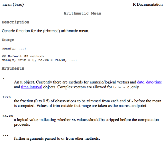
Figure 1. A portion of the R help page about the function mean.
From the help page (Fig 1) we can see that we can specify a trimmed mean by adding options to the mean(x, ...) command. For our x variable defined above, get the trimmed mean after 25% of the data are removed.
mean(x, trim=0.25)[1] 6From the help page we see that the only required option you need to feed the mean command is the name of the variable, in this case, “x” (it can be, of course, any name provided the data are attached). In this case we removed 25% of the values – 12.5% of the smallest values and 12.5% of the largest values – that’s also called the interquartile mean. We use a dot plot to show these trends (Fig 2).
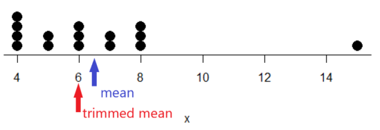
Figure 2. Dot plot of our x variable with locations of the mean (blue) and the trimmed mean (red). The Dotplot(x) function in package RcmdrMisc was used in Rcmdr to make this graphic. Arrows were added by hand. Dotplot() example code presented in Chapter 3.4.
If we recalculate a trimmed mean after dropping 10% of the points, or even 40% of the points, we get the same mean value of 6. The trimmed mean is an example of a robust estimator; it’s resistant to the influence of outliers.
Another useful descriptor of the middle is the geometric mean. The geometric mean is useful for calculating the average of ratios. Geometric mean would be used when you want to compare central tendency for different variables, each differing in scale. For example, gene expression results, reported as fold-changes, for different genes often shows tremendous differences among genes and would be best described by logarithmic scale, not arithmetic scale. Geometric mean expression values would be better choice for central tendency. Other examples are found in economics: for example, calculating compound interest or interest. The geometric mean applies whenever the scale is multiplicative and not additive
The geometric mean is given by the equation

The geometric mean (gm) is equivalent to log-transforming your data, then calculating the arithmetic mean, and transforming the result back (with the antilog exponent.) As you recall, for our simple data set the arithmetic mean was 6.2. The geometric mean for this data was 5.977. Taking the natural log for each of the values from our simple data set, then calculating the arithmetic mean we have 1.788.
The antilog of this value is
exp(1.788)[1] 5.977Another frequently encountered mean is the harmonic mean, which is defined by the equation

Harmonic mean is appropriate for averaging rates. For example, what is the average speed traveled if you travel 30 miles per hour (mph) between point A and B, then on the return trip, your speed was 40 mph? If you think (30 + 40)/2 = 35 mph, then this would be incorrect — after all, the distance covered has not changed, just the time. The harmonic mean returns 34.2 mph. Let
y = c(30,40)The harmonic mean returns 34.2 mph ( see below “How to calculate these other means”)
Both harmonic and geometric means apply for values greater than zero.
How to calculate these “other” means.
In Microsoft Excel, calculate geometric mean via the function GEOMEAN(); calculate harmonic mean via the function HARMEAN().
The base R (and Rcmdr) doesn’t have built in functions for these, although you could download and install some R packages which do (eg, package psych, geometric.mean(variable), harmonic.mean(variable)). It is quicker to just to calculate these by submitting a snippet of code into the script window
For geometric mean of variable “x” at the R prompt type
exp(mean(log(x)))For harmonic mean of variable “x” at the R prompt type
1/mean(1/x)where is the base of the natural logarithm, Euler’s number, and log is the natural logarithm (in R, to get log to other bases you can use log10 for base 10 logarithm or log2 for base 2 logarithm, or log(x, base = n) for any base n of the variable x, and variable is the name of the variable you wish to do the calculations on.
R code: Do try on your own!
Here’s some numbers to try your hand. For example, create a variable containing a few numbers, any numbers. and write it to the variable named z
myZ = c(3,4,6,7,9,11,4)Now, calculate the arithmetic mean, the geometric mean, and the harmonic mean for the variable myZ. You should get Table 4.2)}
Table 2. Comparison of different means for myZ.
| mean | value |
|---|---|
| Arithmetic | 6.285714 |
| Geometric | 5.716403 |
| Harmonic | 5.204936 |
Try three more. In R (or R Commander script window), create three new variables.
varA = c(3,3,3,3)varB = c(1,2,3,12)varC = c(-3,0,1,3)Now, calculate the arithmetic mean, geometric mean, and harmonic mean for each variable.
For the simple arithmetic mean
mean(varA)For the geometric mean, use the formula above
exp(mean(log(varA)))For the harmonic mean, use the formula above
1/mean(1/varA)What did you get?
Other measures of central tendency
Median
The median, which lacks an accepted notation — we’ll go with  , divides a set of observed numbers into two equal halves. Half the observations are above the median, half of the observations are below the median. Arrange data from lowest to highest, take the middle measurement:

odd number of measurements minus the middle value minus even number of measurements minus average of the 2 middle values

Or, more succinctly, we have
![\begin{align*}Med(X) = \left\{\begin{matrix} X\left [ \frac{n+1}{n} \right ] & if \ n \ is \ odd\\ \frac{X\frac{n}{2}+X\frac{n}{2}+1}{2} & if \ n \ is \ even \end{matrix}\right. \end{align*}](https://biostatistics.letgen.org/wp-content/ql-cache/quicklatex.com-9a1a58dc16fffb57b1de96b28c65f0dc_l3.png "Rendered by QuickLaTeX.com")
To get the median in R type at the R prompt
median(variable)and of course, replace variable with the name of the variable containing the numbers. For our x variable created earlier, the function median returns in R
[1] 6[Note that the median for x was the same as the trimmed mean for x, which is consistent with with our view that the trimmed mean is a robust estimator of the middle of a data set.
Mode
Mode is another way to express the middle and it refers to the most frequent occurring measurement. Use of mode makes most sense for discrete or countable numbers. For a normal distribution, the mean, median and mode will be the same value. Note that a data set may have more than one mode. For example, what is the mode for the variable we created earlier?
myX = c(4,4,4,4,5,5,6,6,6,7,7,8,8,8,15)For this small data set we see that “4” is the most frequent with a count of four occurrences in the set.
Mode would seem like a straightforward function in R. However, it turns out there is not a mode function in the base package.
A little explanation is in order. In R, typing mode at the R prompt like so
mode(myX)returns
[1] "numeric" Not the answer we were expecting. In R, mode command is used to tell you what the mode (ie, way or manner in which some task is accomplished) of storage is for the variables.
In order to get the statistical mode we want, we either hunt down a package that contains mode estimation (eg, install the package DescTools use the Mode function — see below), or we can write a little code.
Note 3: A reminder — what we are attempting is to estimate a statistic. DescTools includes about 80 different statistics functions, including functions to calculate every statistic described in this chapter, chapter 3.3, and most other chapters in this book.
A quick Google search found a number of answers at stackoverflow.com (eg, question 2547402). The simplest response was to use names and max commands like so
temp = table(as.vector(myX))names (temp)[temp==max(temp)]Why the median may be a better middle than the mean
Comparing the two measures of central tendency can tell you without plotting how your data are distributed about the middle. Sample distributions are discussed in Chapter 6.
- When the distribution of the data is symmetric or normally distributed (discussed in Chapter 6.7) then the mean and the median will be about the same value
- When data are right-skewed (a few large values), then the mean will be greater than the median.
- When the data are left-skewed (a few small values), then the mean will be less than the median.
Here’s an illustration (Fig 3). I sampled 100 points from a random normal distribution with mean zero and standard deviation 0ne and another 100 points from a log-normal distribution also with mean zero and standard deviation one. In Figure 3, the histograms (see Chapter 4.2 – Histograms), along with summary statistics (see Note 4). Means are indicated with red arrows and medians are indicated with blue arrows.
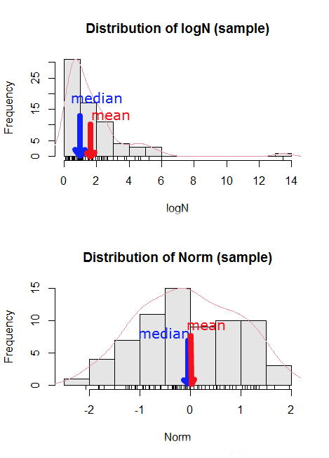
Figure 3. Normal and lognormal distributions with mean (red) and median (blue) noted for comparison.
So the median is a better descriptor or the central tendency of a sample distribution when the distribution is NOT normally distributed.
Note 4: “Summary statistics” refers to reporting of one or more descriptive statistics on a data set. The mean, median, standard deviation, range are common reported statistics. R Commander provides a menu to select from descriptive statistics, returning a table of the estimates. Rcmdr: Statistics → Summaries → Numerical summaries…
Scaling and transformation of data
Sometimes it is useful to standardize your data so that the variables all have the same scale. One algorithm for standardization is called normalization. Normalization implies that you correct the data so that data has a mean, μ, of zero, and a standard deviation, σ, of 1 (unit variance). There are several ways to standardize, each with strengths and limitations. To normalize we use the Z-score equation (see Chapter 6.7 for other uses of Z score).

where Xi is each observation in your data set.
Normalization will make outliers, the few points in a data set that are noticeably different from the central tendency of the rest of the data, smaller and less influential. When you normalize multiple sets of data, then each will have the same mean (0) and variance (unit variance), but the ranges will differ. An example of this is the simple product moment correlation — by standardizing you change the variances for the different variables to have the same unit variance.
As we will see later in class it is also useful to expand or contract the variability of the data or to change the shape of the distribution (if the data is not normally distributed). For example, if you compare individuals of a population for many morphological traits (eg body size, growth rate), the spread of points (called a distribution) will look more like a Poisson distribution (not symmetrical about the mean, a few individuals may be much larger…). This is partly due to the way in which morphological traits are measured. We normally measure body size on a linear scale (inches or centimeters). However, body size is affected by physiological processes that are more related to volume. Therefore, the more appropriate scale of measurement is on a log scale. We can transform the data measured on a linear scale to a log scale. For morphological traits this can produce a distribution that is normally distributed (bell shape). There are many more statistical procedures for data that is normally distributed than there are statistical procedures for Poisson distributions or any other type of distribution. Additional discussion about data transformation is introduced in Chapter 13.3.
You can always uncode or unstandardize your data after performing the statistical procedures and return to the original scale. In fact, when reporting descriptive statistics you should report the untransformed, uncoded data. Moreover, you will find it useful to report means adjusted for other variables (eg, from ANOVA or regression); if the ANOVA or regression equations are performed on transformed or coded data you would want to back calculate to the original scale after applying the ANOVA or regression adjustments. This advise will make more sense after we’ve discussed ANOVA (Chapter 12) and linear regression (Chapter 17).
R operators
The names command can be used to retrieve the names contained in the variable (if text types) or to set the names of the observations, which is what we are using it for here. We set the numbers to text names “4”, “5”, etc. then find the maximum count of named items in the temp table. The double equals operator (==) is used to tell R to find the object that is “equal to” something we specify, in this case, the max value (R Language Definition 2014). Table 3 shows common operators in R.
Table 3. Common arithmetic* and comparison** operators
| Operator | Description |
|---|---|
| ? | help |
| + | plus |
| - | minus |
| * | multiply |
| / | divide |
| : | series |
| > | greater than |
| < | less than |
| >= | greater than or equal to |
| <= | less than or equal to |
| = | left assignment |
| <- | left assignment |
== | equal to |
** To list and get help with use of comparison operators enter at the R prompt
help(Arithmetic)
help(Comparison)
The R package modeest has a number of algorithms for calculating the mode, depending on the kind of data you are working with. After installing the package and its dependencies, type at the R prompt
require(modeest)
mfv(myX)
[1] 4
Creating objects in R
Everything in R is an object (Chambers 2008). We provide many worked examples in Part 07. Working with your own data – Mike’s Workbook for Biostatistics. In brief, create a variable in R by assigning the vector x, either directly at the R prompt or in a script window (Rcmdr, RStudio), like so
myX = c(4,4,4,4,5,5,6,6,6,7,7,8,8,8,15)
The function c(), which stands for combine is used to combine the set of numbers into the object, myX. For small sets like this you may find it convenient to enter the values one by one and let R store it into the vector for you. For R installed on your computer, use the scan() function and your keyboard — scan() doesn’t work consistently in serverless R instances (eg., Google CoLab). Careful! Make sure that you remember to assign the results from scan to a vector.
I’ll create the object tryScan just to distinguish it from x, although I will enter the same values. Until R receives an interrupt signal from you, it will prompt you to enter numbers one row at a time. When you’ve reached the end, use the keyboard shortcut Ctrl + q (Windows) or Cmd + q (macOS) to interrupt keyboard input.
tryScan = scan()
1: 4
2: 4
3: 4
4: 4
5: 5
6: 5
7: 6
8: 6
9: 6
10: 7
11: 7
12: 8
13: 8
14: 8
15: 15
Read 15 items
tryScan
 [1] 4 4 4 4 5 5 6 6 6 7 7 8 8 8 15
The function tryScan is a very useful command, with many options, and can be used for more than keyboard entry. For example, you can paste from your computer’s clipboard a column of numbers from your spreadsheet.
R code calculate central tendency
Once we have the vectormyX, calculate the mean by entering at the R prompt
mean(myX)
and you should get the answer of 6.466667
And of course, you don’t type in the R prompt >, right?
Or, for the better option, create two variables, one containing the list of observed numbers and the second that contains the frequency for each observed number in the series. You would then use the command for weighted mean.
myY = c(4,5,6,7,8,15)
myW = c(4/15, 1/15, 3/15, 2/15, 4/15, 1/15)
Note — you can check that the frequencies sum to 1 by using the sum command like so
sum(myW)
For the weighted mean, the command is
weighted.mean(myY,myW)
and, the answer returned is 6.466667, the same as before.
There’s an R package for that.
We list code examples for all of the statistics described on this page, but as you can imagine, there are packages that include these and other useful functions, or “wrapper functions” that make writing code easier in R. A good example is the DescTools package. One advantage of using a package like DescTools is that it cuts through the need to remember specific commands for basic data exploration. For example, just call the Desc() function to yield several measures of central tendency and dispersion (see Chapter 3.3).
The R code and output follows, along with a plot (Fig 4). The mean and median are highlighted in orange.
Desc(myX)
────────────────────────────────────────────────────────────────────────────────
myX (numeric)

length      n   NAs unique   0s  mean meanCI'
    15     15     0      6    0  6.47    4.92
       100.0%  0.0%        0.0%          8.02

   .05    .10   .25 median  .75   .90     .95
  4.00   4.00  4.50   6.00 7.50  8.00   10.10

range      sd vcoef    mad  IQR  skew    kurt
11.00    2.80  0.43   2.97 3.00  1.72    2.94

  value freq   perc cumfreq cumperc
1     4    4  26.7%       4   26.7%
2     5    2  13.3%       6   40.0%
3     6    3  20.0%       9   60.0%
4     7    2  13.3%      11   73.3%
5     8    3  20.0%      14   93.3%
6    15    1   6.7%      15  100.0%

' 95%-CI (classic)

Figure 4. Histogram, box plot, and cumulative distribution function plot generated by default by Desc() call.
Lots of output! This is a good example of how to explore data — describe the middle (eg, mean and median), but also the variability about the middle (eg, range, standard deviation — sd, mean absolute deviation — mad, coefficient of variation — vcoef), and distribution shape (quantiles — 0.05, 0.25 etc, kurt, skew). The plots — histogram, box plot, and cumulative distribution plots — are explained in Chapter 4.
Use aggregate() to calculate summary statistics by group.
So far, all code presumes need to calculate descriptive statistics one vector at a time. In general, we need summary statistics for more than one group or strata. For example, we may ask, what are the average body temperature readings measured by IR device on different body areas from several subjects (question 8a, Homework 2A: Descriptive statistics in Mike’s Workbook for Biostatistics).
The aggregate() function in R simplifies calculating means by groups by providing a concise and efficient way to apply a summary function (like mean()) to a variable, grouped by one or more other variables. The format for aggregate is
aggregate(x = variable_to_aggregate ~ grouping_variable, FUN = mean, data = your_dataframe)
Questio8a had two levels of body regions, “Forehead” and “Throat.” Assuming the variable is named bodyTemp and the grouping variable is called bodyGroup and stored in the attached data.frame question08a, then the following R code provides the requested summary statistics by groups.
aggregate(bodyTemp ~ bodyGroup, data = question08a,
function(x) c(mean = mean(x)))
Additional statistics can be requested by adding one after the other following mean(x), eg, median = median(x).
Note 5: aggregate() is part of the base R installation. Additional functions are available, including dplyr and data.table packages, which the user is encouraged to explore!
The advantage of use of R Commander, it’s easy to get multiple statistics by groups by following the drop down menus, beginning with Statistics > Summaries > Table of statistics… (Fig 5).

Figure 5. Screenshot R Commander, summary statistics by group.
Questions
- Find the help page in R for the median function. How does the function handle missing values?
- For a simple data set like the following
myY <- c(1,1,3,6)you should now be able to calculate, by hand, the
• mean • median • mode - If the observations for a ratio scale variable are normally (symmetrically) distributed, which statistic of central tendency is best (eg, less sensitive to outlier values)?
- In the
names()command, what do you think the result will be if you replacemaxin the command withmin? - If data are right skewed, what will be the order of the mean, median, and mode?
- Body mass of Rhinella marina (formerly Bufo marinus, Fig 6),
bufo <- c(71.3, 71.4, 74.1, 85.4, 85.4, 86.6, 97.4, 99.6, 107, 115.7, 135.7, 156.2)

Figure 6. Female Rhinella marina (formerly Bufo marinus), Chaminade University campus. Body length 23.5 cm. Click image to view full sized image.
- Under what circumstances is it appropriate to transform raw data?
- What does “standardize” or “normalize” imply as actions to take with data?
Quiz Chapter 3.2
Measures of Central Tendency
Chapter 3 contents
- Exploring data
- Data types
- Measures of Central Tendency
- Measures of dispersion
- Estimating parameters
- Statistics of error
- References and suggested readings