16.6 – Similarity and Distance
Introduction
A measure of dependence between two random variables. Unlike Pearson Product Moment correlation, distance correlation measures strength of association between the variables whether or not the relationship is linear. Distance correlation is a recent addition to the literature, first reported by Gábor J. Székely (e.g., Székely et al. 2007). The package correlation (Makowski et al 2019) offers distance correlation and significance test.
Example, fly wing dataset introduced 16.1 – Product moment correlation
library(correlation)
Area <- c(0.446, 0.876, 0.390, 0.510, 0.736, 0.453, 0.882, 0.394, 0.503, 0.535, 0.441, 0.889, 0.391, 0.514, 0.546, 0.453, 0.882, 0.394, 0.503, 0.535)
Length <- c(1.524, 2.202, 1.520, 1.620, 1.710, 1.551, 2.228, 1.460, 1.659, 1.719, 1.534, 2.223, 1.490, 1.633, 1.704, 1.551, 2.228, 1.468, 1.659, 1.719)
FlyWings <- data.frame(Area, Length)
correlation(FlyWings,method="distance")
Output from R
# Correlation Matrix (distance-method)
Parameter1 | Parameter2 |    r |       95% CI | t(169) |      p
------------------------------------------------------------------
      Area |     Length | 0.92 | [0.80, 0.97] |  30.47 | < .001***

p-value adjustment method: Holm (1979)
Observations: 20
The product-moment correlation was 0.97 with 95% confidence interval (0.92, 0.99). The note about “p-value adjustment method: Holm (1979)” refers to the algorithm used to mitigate the multicomparison problem, which we first introduced in Chapter 12.1. The correction is necessary in this context because of how the algorithm conducts the test of the distance correlation. Please see Székely and Rizzo (2013) for more details.
Which should you report? For cases where it makes sense to test for a linear association, then the Product-moment correlation is the one to use. For other cases where no inference of linearity is expected, then the distance correlation makes sense.
Similarity and Distance
Similarity and distance are related mathematically. When two things are similar, the distance between them is small; When two things are dissimilar, the distance between them is great. Whether similarity (sometimes dissimilarity) or distance, the estimate is a statistic. The difference between the two is that the typical distance measures one sees in biostatistics all obey the triangle inequality rule while similarity (dissimilarity) indices do not necessarily obey the triangle inequality rule.
Distance measures
Distance is a way to talk about how far (or how close) two objects are from each other (Fig. 1). The distance may be relate to physical distance (map distance), or in mathematics, distance is a metric or statistic. Euclidean distance is the distance between two points in either the X-Y plane or 3-dimensional space measures the length of a segment connecting the two points (e.g., x1,y1 = 1, 4 and x2,y2 = 1,4).
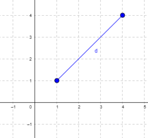
Figure 1. Cartesian plot of two points, the first at x1 = 1 and y1 = 1 and the second at x2 = 4 and y2 = 4.
For two points (x1, y1 and x2, y2) described in two dimensions (e.g., an xy plane), the distance d is given by

For two points described in three (e.g., an xyz-space), or more dimensions, the distance d is given by

Distances of this form are Euclidean distances and can be directly obtained by use of the Pythagorean Theorem. The triangle inequality rule then applies (i.e., the sum of any two sides must be less than the length of the remaining side). Euclidean distance measures also include
- Manhattan distance: the sum of absolute difference between the measures in all dimensions of two points.

- Chebyshev distance: also called the maximum value distance, the distance between two points is the greatest of their differences along any coordinate dimension.

Note: We first met Chebyshev in Chapter 3.5.
Example
There are a number of distance measures. Let’s begin discussion of distance with geographic distance as an example. Consider the distances between cities (Table 1).
Table 1. Distances (miles) among cities.
| Honolulu | Seattle | Manila | Tokyo | Houston | |
| Honolulu | 0 | 2667.57 | 5323.37 | 3849.99 | 3891.82 |
| Seattle | 2667.57 | 0 | 6590.23 | 4776.81 | 1888.06 |
| Manilla | 5323.37 | 6590.23 | 0 | 1835.1 | 8471.48 |
| Tokyo | 3849.99 | 4776.81 | 1835.1 | 0 | 6664.82 |
| Houston | 3891.82 | 1888.06 | 8471.48 | 6664.82 | 0 |
This table is a distance matrix — note that along the diagonal are “zeros,” which should make sense — the distance between an object and itself is, well zero. Above and below the diagonal you see the distance between one city and another. This is a special kind of matrix called a symmetric matrix. Enter the distance in miles (1 mile = 1.609344) between 2 cities (this is “pairwise“). There are many resources “out there,” to help you with this. For example, I found a web site called mapcrow that allowed me to enter the cities and calculate distances between them.
To get the distance matrix, use this online resource, the Geographic Distance Matrix Calculator.
Real world problem, use geodist package. Provide latitude and longitude coordinates
The dist() function in R base will return Manhattan distance and others () on matrices.
R script
HNL <- c(0, 2667.57, 5323.37, 3849.99, 3891.82)
SEA <- c(2667.57, 0, 6590.23, 4776.81, 1888.06)
MAN <- c(5323.37, 6590.23, 0, 1835.1, 8471.48)
TOK <- c(3849.99, 4776.81, 1835.1, 0, 6664.82)
HOU <- c(3891.82, 1888.06, 8471.48, 6664.82, 0)
mat.city <- rbind(HNL, SEA, MAN, TOK, HOU)
colnames(mat.city) <- c("HNL", "SEA", "MAN", "TOK", "HOU")
mat.city
dist(mat.city, method = "manhattan")
R output
        HNL       SEA     MAN      TOK
SEA 9532.58
MAN 21163.95 25361.39
TOK 16070.49 20267.93 8763.66
HOU 14526.09 8769.63 27906.40 22896.60
Other distances, replace “manhattan” with
For example,
dist(mat.city, method = "euclidean")
R output
         HNL       SEA     MAN       TOK
SEA 4550.917
MAN 9853.774 12079.347
TOK 7345.155 9615.750 3931.736
HOU 6980.976 3966.360 13820.922 11883.931
The Chebyshev distance doesn’t seem to be part of base R, but is available in other packages (philentropy, function distance).
Note 1. Need a different distance measure? Chances are philentropy packages can calculate it; use getDistMethods() to explore available measures.
R script
require(philentropy)
distance(mat.city, method = "chebyshev", diag=FALSE, upper=FALSE)
R output
     v1         v2      v3      v4      v5
v1    0.00 2667.57 5323.37 3849.99 3891.82
v2 2667.57    0.00 6590.23 4776.81 1888.06
v3 5323.37 6590.23    0.00 1835.10 8471.48
v4 3849.99 4776.81 1835.10    0.00 6664.82
v5 3891.82 1888.06 8471.48 6664.82    0.00
Distance measures used in biology
It is easy to see how the concept of genetic distance between a group of species (or populations within a species) could be used to help build a network, with genetically similar species grouped together and genetically distant species represented in a way to represent how far removed they are from each other. Here, we speak of distance as in similarity: two species (populations) that are similar are close together, and the distance between them is short. In contrast, two species (populations) that are not similar would be represented by a great distance between them. Genetic distance is the amount of divergence of species from each other. Smaller genetic distances reflects close genetic relationship. Hamming distance is a common choice, good for categorical data.
Here’s an example (Fig. 2), RAPD gel for five kinds of beans. RAPD stands for random amplified polymorphic DNA.
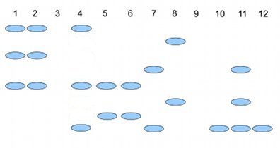
Figure 2. RAPD gel (simulated) five kinds of beans.
Samples were small red beans (SRB), garbanzo beans (GB), split green pea (SGP), baby lima beans (BLB), and black eye peas (BEP). RAPD primer 1 was applied to samples in lanes 1 – 6; RAPD primer 2 was applied to samples in lane 7 – 12. Lane 1 & 7 = SRB; Lane 2 & 8 = GB; Lanes 3 & 9 = SGP; Lane 4 & 10 = BLB; Lane 5 & 11 = BB; Lane 6 & 12 = BEP.
Here’s how to go from gel documentation to the information needed for genetic distance calculations (see below). I’ll use “1” to indicate presence of a band, “0” to indicate absence of a band, and “?” to indicate no information. For simplicity, I ignored the RF value, but ranked the bands by order of largest (= 1) to smallest (=8) fragment.
We need three pieces of information from the gel to calculate genetic distance.
NA = the number of markers for taxon A
NB = the number of markers for taxon B
NAB = the number of markers in common between A and B (this is the pairwise part — we are comparing taxa two at a time.
First, compare the beans against the same primer. My results for primer 1 are in Table 2; results for primer 2 are in Table 3.
Table 2. Bands for Primer 1
| marker | lane 1 | Lane 2 | Lane3 | Lane 4 | Lane 5 | Lane 6 |
| 1 | 1 | 1 | ? | 1 | 0 | 0 |
| 3 | 1 | 1 | ? | 0 | 0 | 0 |
| 5 | 1 | 1 | ? | 1 | 1 | 1 |
| 7 | 0 | 0 | ? | 0 | 1 | 1 |
Table 3 for Primer 2
| marker | Lane 7 | Lane 8 | Lane 9 | Lane 10 | Lane 11 | Lane 12 |
| 2 | 0 | 1 | ? | 0 | 0 | 0 |
| 4 | 1 | 0 | ? | 0 | 1 | 0 |
| 6 | 0 | 1 | ? | 0 | 1 | 0 |
| 8 | 1 | 0 | ? | 1 | 1 | 1 |
From Table 2 and Table 3, count NA (= NB ) for each taxon. Results are in Table 4.
Table 4. Bands for each taxon.
| Taxon | No. markers from Primer1 |
No. markers from Primer2 |
Total |
| SRB | 3 | 2 | 5 |
| GB | 3 | 2 | 5 |
| SGP | ? | ? | ? |
| BLB | 2 | 1 | 3 |
| BB | 2 | 3 | 5 |
| BEP | 2 | 1 | 3 |
To get Hamming distance between SRB and BB (from Table 2 and Table 3), R script as follows.
SRB <- c(1, 1, 1, 0, 0, 1, 0, 1)
GB <- c(0, 0, 1, 1, 0, 1, 1, 1)
# sum the inequality between the two vectors
sum(SRB != GB)
R output
> sum(SRB != GB)
[1] 4
Hamming distance between small red beans and black beans for the markers is 4.
Note 2. h/t https://www.r-bloggers.com/2021/12/how-to-calculate-hamming-distance-in-r/
As you can see, there is no simple relationship among the taxa; there is no obvious combination of markers that readily group the taxa by similarity. So, I need a computer to help me. I need a measure of genetic distance, a measure that indicates how (dis)similar the different varieties are for our genetic markers. I’ll use a distance calculation that counts only the “present” markers, not the “absent” markers, which is more appropriate for RAPD. I need to get the NAB values, the number of shared markers between pairs of taxa.
Table 5. NAB
| SRB | GB | BLB | BB | BEP | |
| SRB | 0 | 3 | 3 | 3 | 2 |
| GB | 0 | 2 | 2 | 1 | |
| BLB | 0 | 2 | 2 | ||
| BB | 0 | 3 | |||
| BEP | 0 |
The equation for calculating Nei’s distance is:

where NA = number of bands in taxon “A”, NB = number of bands in taxon “B”, and NAB is the number of bands in common between A and B (Nei and Li 1979). Here’s an example calculation.
Let A = SRB and B = GB, then

The R package adegenet includes Nei’s distance (and others), but the data set assumes more information than I provided here (e.g., ploidy, alleles).
Which distance measure to use?
Unfortunately, not a simple answer. A quick search of journals will likely return “Euclidean distance” the most common (Evolution = 328, Ecology = 298). The different distance (similarity) measures were developed to solve sometimes related, but often different problems, and so a review of the statistical properties would be warranted before making a choice. Helpful reviews
Questions
1. Write up three learning outcomes for this page. Hint: Point your favorite generative AI to this page and ask for help.
2. Review all of the different correlation estimates we introduced in Chapter 16 and construct a table to help you learn. Product moment correlation is presented as example.
| Name of correlation | variable 1 type | variable 2 type | purpose |
| Product moment | ratio | ratio | estimate linear association |
3. Be able to define and distinguish between similarity measures, dissimilarity measures quantify, and distance.
4. Return to our counts of colored candies from mini bags of Skittles, M&M plain chocolate, and M&M peanut. Which two are most similar? Here’s a data sample. Calculate the Euclidean pairwise distances, then the Manhattan distances among the bags of candies. Do you get the same answer?
The data
| Color | Skittles | mm_plain | mm_peanut |
|---|---|---|---|
| Blue | 0 | 19 | 18 |
| Green | 40 | 43 | 28 |
| Yellow | 30 | 29 | 9 |
| Orange | 26 | 39 | 18 |
| Red | 28 | 15 | 4 |
| Purple | 28 | 0 | 4 |
| Brown | 0 | 16 | 0 |
Example R code
Note 3. The code works. Remember, sometimes when copying code from a website you pickup additional characters. While every effort has been made to provide clean html — if you run into problems, chances are the simplest fix is to type the code fresh rather than trying to figure out why the copied code fails.
mySites <- data.frame(
Site <- c("A","B","C"),
Spp1 <- c(10, 5, 12),
Spp2 <- c(7, 15, 8),
Spp3 <- c(3, 2, 9)
)
# View the matrix
print(mySites)
# Exclude the "Site" column
myAbundances = mySites[,-1]
# Calculate the Euclidean distance matrix
dist(myAbundances,method="euclidean")
The output should be
          1          2
2  9.486833
3  6.403124  12.124356
where “1” refers to site A, “2” refers to site B, and “3” refers to site C. We would conclude that sites A and C are most similar, or have similar species abundance, because they have the smallest Euclidean distance. As you can imagine, there’s more to interpreting these statistics, and in particular, Euclidean distance can lead to some confusing interpretations about abundance and species composition between sites, eg, Orlóci paradox. Interested readers should see Ricotta 2021.
Note 4. Orlóci paradox refers to a problem with Euclidean distances: two sites with no species in common may be interpreted as more similar that two sites that share the same species. This is because Euclidean distance is more sensitive to abundance than presence/absence.
Why then teach Euclidean distance? The Euclidean distance is a standard measure, it helps lay the foundation for understanding geometric concepts. Its limitations are a reminder that students need to be aware that alternative methods are sometimes needed.
Quiz Chapter 16.6
Similarity and Distance