3.4 – Estimating parameters
Introduction.
What you will find on this page. Definitions for constants, variables, and parameters as used in data analytics. Statistical bias and the concept of unbiased estimators are discussed. The different types of error are introduced along with definitions of accuracy and precision. Statistics used to quantify error are presented in the next section, Chapter 3.4.
Estimating parameters.
Parameters belong to populations; they are fixed but unknown. Parameters are characteristics of populations: the typical average height and weight of five year old children; What is the normal range of values for height and weight of five year old children; average and range of gene expression of TP53 in epithelial lung cells of 50 year old non-smoking humans; etc. Because we generally do not have at our disposal surveys — census — of entire populations for these characteristics, we sample and calculate descriptive statistics for a subset of individuals from populations: these statistics, the mean height, range of height, etc., are variables. We expect average height, range of height, etc., to change, to vary, from sample to sample. A constant, as the word implies, is not variable and remains unchanged.
We estimate parameters (means, variances) from samples of observations from a population. Intuitively then, our estimates are only as good as how representative of the population the sample is. Statistics allows us to be more precise: we can define “how good” our estimates are by asking about, and quantifying, the accuracy and precision of our estimates.
Notwithstanding the notion of “personalized medicine,” our goal in science is to understand cause and effect among sets of observations on samples from a population. We ask, what is the link between lung cancer and smoking? We know that smoking tobacco cigarettes increases risk of cancer, but not everyone who smokes will get cancer (Pesch et al., 2012). Tumorigenic risk is in part mediated by heredity (cf. Trifiletti et al 2017). That’s one way we run into problems in statistics: the biological phenomenon is complicated in ways we are not yet aware of, and thus samples drawn from populations are heterogeneous. Put another way, we think there is one population, but there may be many distinct populations. By chance, repeated samples drawn from the population include individuals with different risk associated with heredity.
As an aside, this is precisely why the concept of personalized medicine is important. Medical researchers have learned that some people with breast cancer respond to treatment with trastuzumab, a monoclonal antibody, but others do not (review in Valabrega et al 2007). Responders have more copies of a gene, copy number variation, for an EGF-like receptor called HER2. In contrast, non-responders to trastuzumab have fewer copies of this receptor (and are said to be HER2-negative in an antibody test for HER2). Thus, we speak about people with breast cancer as if the disease is the same, and from a statistical point of view, we would assume that individuals with breast cancer are of the same population. But they are not — and so the treatment fails for some, but works for others. In this example, we have a mechanism or cause to explain why some do not respond; their breast cancer is not associated with increased copy numbers of HER2. And so in studies with breast cancer, statisticians may account for differences in HER2 status. Note: Fewer than 30% of breast cancer may have over-expression of HER2, (Bilous et al. 2003).
Clearly, HER2 status would be used by statisticians when drawing samples from population, and we would not mistake samples. But, in many other situations we are not aware of any differences and so we assume our samples come from the same population. Note that even with imperfect knowledge about samples, experimental design is intended to help mediate heterogeneous samples. For example, this is why treatment controls need to be used, or case controls are included in studies.
Random assignment to groups also is an attempt to control for unknowns: if random, then all treatment groups will likely include representatives of the numerous co-factors that contribute to risk.
Statisticians have an additional, technical burden: there are often a variety of ways (algorithms) to describe or make inferences about samples, and they are not equally capable of giving us “truth.” Estimates of a parameter are not going to be exactly the true value of the parameter! This is the problem of identifying unbiased ways to estimate parameters. In statistics, bias quantifies whether an algorithm to calculate a particular statistic (e.g., the mean or variance), is consistently too low or too high.
Random sampling.
Random sampling from the population is likely to be our best procedure for obtaining representative samples, but it is not foolproof (we’ll return to situations where random sampling fails to provide adequate samples of populations in Chapter 5.5 Importance of randomization in experimental design). However, a second concern is how to calculate the mean, how to calculate the variance. In the section on Descriptive Statistics (Chapter 3.2), we presented how to calculate the arithmetic mean — the simple average — but also introduced you to other calculations for the middle (e.g., median, geometric mean, harmonic mean). How to know which “middle” is correct?
Statisticians use the concept of bias — the simple arithmetic mean is an unbiased estimator of the population parameter, but a correction needs to be made to the calculation of sample variance to remove bias. Bias implies that the estimator systematically misses the target in some way. Good or “best” parameter estimates are, on average, going to be close to the actual parameter if we collected many samples of the population (this will depend on the sample size and the variability of the data). Earlier we introduced Bessel’s correction to the sample variance, divide the sum of squares by n – 1 and not N as we did for the population variance, so that it is an unbiased estimator of the sample variance. Thus, statisticians have worked out how well their statistical equations work as estimators; concepts of expected values or the expectation are used to evaluate how well an estimator works. In statistics, the expected value of a statistic is calculated by multiplying each of the possible outcomes by the likelihood each outcome will occur and then summing all of those values..
We need to add a bit more to our discussion about measurement and estimation.
Types of error.
To measure is to assign a number to something, a variable. Measurements can have multiple levels, but are of the four data types: nominal, ordinal, interval scale, and ratio scale. Nominal and ordinal types are categorical or qualitative; interval and ratio are continuous or quantitative. Errors in measurement represent differences between what is observed and recorded compared with the true value, i.e., the actual population value. With respect to measurement we distinguish between random errors and systematic errors. Random errors occur by chance, and are thus expected to vary from one measurement instance from another. Random error may lead to measures larger or smaller than the true value. Systematic errors are of a kind that can be attributed to failures of an experimental design or instrument.
Accuracy is reflected in the question: how close to the true value is our measure? Accuracy is distinct from precision, the concept of how clustered together are repeated values for the same measurement. All measurement has associated error, which may be divided into two kinds: random error and systematic error.
We tend to think of error in terms of mistakes, mistakes by us or as failure of the measurement process. However, in biology research, that is too restrictive of a meaning for error. First, experimental error occurs when the estimates derived from the samples — sample mean, sample variance — differ from the population parameters — population mean, population variance. Second, error in biology ranges from mistakes in data collection to real differences among individuals for a characteristic. The latter source, error among individuals, is of course, not a mistake, but rather, it’s the “very spice of life” (Cowper 1845). We’ll leave the study of individual differences, biological error, for later. This section is concerned with error in the sense of mistakes.
Random error includes things like chance error in an instrument leading to different repeat measures of the same thing and to the reality that individual differences exist for most biological traits. We minimize the effects of this kind of error by randomizing: we randomly select samples from populations; we randomly assign samples to treatment groups. Random error can make it hard to differentiate treatment effects. Random error decreases precision, the repeatability of measures. At worse, random error is conservative — it tends to mean we miss group differences, we conclude that the treatment (e.g., aspirin analgesics) has no effect on the condition (e.g., migraines). This kind of error is referred to as a Type II error (Chapter 8).
The experimental design remedy for random error is to increase sample size, a key conclusion drawn from power analysis on experiments, discussed in Chapter 11. The other type of error, systematic error, a type of bias, is more in line with the idea of errors being synonymous with mistakes. Uncalibrated instruments yield incorrect measures. And these kinds of errors lead us to make errors that can be more problematic. An example? Back in the early 1990s when I started research on whole animal metabolic rates (e.g., Dohm et al 1994, Beck et al 1995), we routinely set baseline carbon dioxide, CO2, levels to 0.035% of volume of dry air (350 ppm, parts per million), which reflected ambient levels of CO2 at the time (see Figure 4 in Chapter 4.6).
#NOAA monthly data from Mauna Loa Observatory
co2.1994 <- c(358.22, 358.98, 359.91, 361.32, 361.68, 360.80, 359.39, 357.42, 355.63, 356.09, 357.56, 358.87)
You are probably aware, today, background CO2 have increased considerably even since the 1980s. Data for 2021 (average 420 ppm — reporting just 2 significant figures) are provided below
co2.2021 <- c(415.49, 416.72, 417.61, 419.01, 419.09, 418.93, 416.9, 414.42, 413.26, 413.9, 414.97, 416.67)
source: Global Monitoring Lab, NOAA
Thus, if I naively compared rates of CO2 produced by an animal at rest,  , measured today against the data I gathered back in the 1990s without account for the change in background CO2 in my analysis, I will have committed a systematic error: values of on animals would be systematically higher than values for 1988 when I apply a baseline correction.
Examples of error.
One under-reported cost of next-generation sequencing technologies is that base calls, the process of assigning a nucleotide base to chromatogram peaks has more errors than traditional Sanger-based sequencing methods (Fox et al 2014). In “next-generation-sequencing” (NGS) methods, individual DNA fragments are assigned sequences, whereas Sanger methods took the average sequence of a collection of DNA fragments; thus, in principle, NGS methods should be able to characterize variation of mixtures of sequences in ways not available to traditional sequencing approaches. However, artifacts introduced in sample preparation and PCR amplification lead to base calling errors (Fox et al 2014).
Gene expression levels will differ among tissue types, thus mixed samples from different tissues will misrepresent gene expression levels.
Measurement of energy expenditure, oxygen uptake and carbon dioxide release by an organism, have long been sources of study in ecology and other disciplines. A classic measure is called basal metabolic rate, measured as the rate of oxygen consumption of an endothermic animal, post-absorptive (i.e., not digesting food), at rest but not sleeping, while the animal is contained within a thermal-neutral environment (Blaxter 1989).
Accuracy and precision.
Two properties of measurement are the accuracy of the measure and its precision. Accuracy is defined as the closeness of a measured value to its true value. Precision refers to the closeness of a second measure to the first, to the closeness of a third measure to the first and second, and so on. Precision refers to repeatability of measurement. We suggested use of the coefficient of variation, defined with examples in Chapter 3.2, as a way to quantify precision.
Consider the accuracy and precision of three volumetric pipettors: p1000, which has a nominal range between 100 and 1000 μL (microliters); p200, which has a range between 20 and 200 μL; p100, which has a range between 10 and 100 μL. Which of these three pipettors do you think would have the best accuracy and precision for dispensing 100 μL? We can test pipettors by measuring the mass of distilled water dispensed by the pipettor on an analytical balance. For 100 μL of distilled water at standard temperature and pressure conditions, the mass of the water would be 0.100 grams. The results are shown in the table, and a dot plot is shown in the figure to help us see the numbers.
Table 1. Mass (grams) of 100 μL of distilled water dispensed by three volumetric pipettors*
| p1000 | p200 | p100 | |
| 0.113 | 0.100 | 0.101 | |
| 0.114 | 0.100 | 0.100 | |
| 0.113 | 0.100 | 0.100 | |
| 0.115 | 0.099 | 0.101 | |
| 0.113 | 0.100 | 0.101 | |
| 0.112 | 0.100 | 0.100 | |
| 0.113 | 0.100 | 0.100 | |
| 0.111 | 0.100 | 0.100 | |
| 0.114 | 0.101 | 0.101 | |
| 0.112 | 0.100 | 0.100 | |
| mean: | 0.113 | 0.100 | 0.1004 |
| standard deviation: | 0.0012 | 0.0005 | 0.0005 |
*Temperature 21.5 °C, barometric pressure 76.28 cm mercury (elevation 52 meters). Data presented in Table 1 were not corrected to standard temperature or pressure.
Here is the code for the R run; assuming that you have started R commander, then copy and paste each line into the R Commander script window; if not, enter the script one line at a time in the R console. Recall that the hashtag, #, is used to add comment lines.
Note 1: A reminder: Don’t include the last two rows from Table 1 in your data set; these contain descriptive statistics and are not your data.
#create the variables
p1000 <- c(0.113, 0.114, 0.113, 0.115, 0.113, 0.112, 0.113, 0.111, 0.114, 0.112)
p100 <- c(0.101, 0.1, 0.1, 0.101, 0.101, 0.1, 0.1, 0.1, 0.101, 0.1)
p200 <- c(0.1, 0.1, 0.1, 0.099, 0.1, 0.1, 0.1, 0.1, 0.101, 0.1)
#create a data frame
pipet <- data.frame(p100,p200,p1000)
attach(pipet)
#stack the data
stackPipet <- stack(pipet[, c("p100","p200","p1000")])
#Add variable names
names(stackPipet) <- c("mass", "pipet")
#create the dot plot
with(stackPipet, RcmdrMisc::Dotplot(mass, by=pipet, bin=FALSE))
From Table 1 we see that the means for the p100 and p200 were both close to the target mass of 0.1 g. The mean for the p1000, however, was higher than the target mass of 0.1 g. A dot plot is a good way to display measurements (Fig. 1).
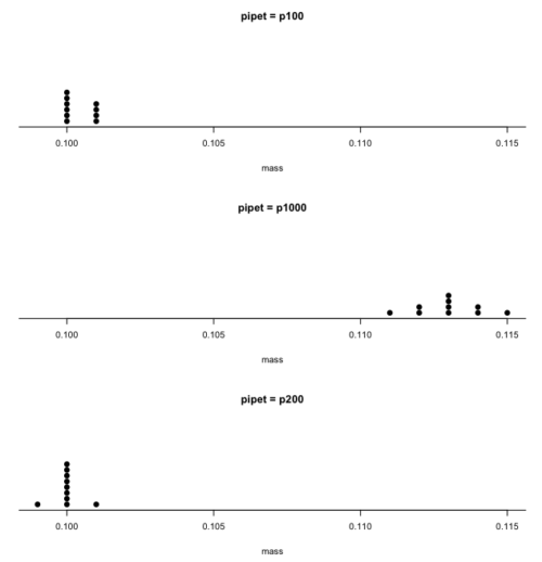
Figure 1. Dot plot of pipet results.
Note 2: Dotplot() is part of the RcmdrMisc package; if you are using the Rcmdr script window (please do!), then the functions in RcmdrMisc are already available and you wouldn’t need to use RcmdrMisc:: (package name plus double-colon operator) to call the Dotplot() function (more properly, referred to as namespaces). Thus, with(stackPipet, Dotplot(mass, by=pipet, bin=FALSE)) would work perfectly well within the Rcmdr script window.
From the dot plot we can quickly see that the p1000 was both inaccurate (the data fall well above the true value), and lacked precision (the values were spread about the mean value). The other two pipettors showed accuracy and looked to be similar in precision, although only two of ten values for the p200 were off target compared to four of ten values for the p100. Thus, we would conclude that the p200 was best at dispensing 100 microliters of water.
In the next chapter we apply statistics to estimate our confidence in this conclusion. In contrast to measurement, estimation implies calculation of a value. In statistics, estimates may be a point, e.g., a value of a collection of data, or an interval, e.g., a confidence interval.
Summary.
This is your first introduction into the concept of experimental design, as defined by statisticians! One of the key tasks for a statistical analyst is to have an appreciation for measurement accuracy and precision as established in the experiment. Precise and accurate measurement levels determine how well questions about the experiment can be answered. At one extreme, if a measure is imprecise, but accurate, then it will be challenging to quantify differences between a control group and a treatment group. At the other extreme, if the measure is precise, but inaccurate, the danger would be differences between the treatment and control group may be more likely, even when the groups are truly not different!
Questions.
- List the types of error in measuring mRNA expression levels on a gene for a sampling of cells from biopsy of normal tissue and a biopsy of a tumor. Assume use of NEXGEN methods for measuring gene expression. Distinguish between technical errors and biological errors.
- If confidence interval are useful for estimating accuracy, what statistic do we call to quantify precision?
Quiz Chapter 3.4
Estimating parameters
Chapter 3 contents