16.1 – Product moment correlation

Introduction
The correlation coefficient
Effect size
Standard error of the correlation
Confidence interval
Significance testing
R code
Assumptions of the product-moment correlation
Testing two independent correlations
Questions
Chapter 16 contents

Introduction

A correlation is used to describe the direction $\pm$ magnitude of linear association and the between two variables. There are many types of correlations, some are based on ranks, but the one most commonly used is the product-moment correlation (r). The Pearson product-moment correlation is used to describe association between continuous, ratio-scale data, where “Pearson” is in honor of Karl Pearson (b. 1857 – d. 1936).

There are many other correlations, including Spearman’s and Kendall’s tau (τ) (Chapter 16.4) and ICC, the intraclass correlation (Chapter 12.3 and Chapter 16.4).

The product moment correlation is appropriate for variables of the same kind — for example, two measures of size, like the correlation between body weight and brain weight.

Spearman’s and Kendall’s tau correlation are nonparametric and would be alternatives to the product moment correlation. The intraclass correlation, or ICC, is a parametric estimate suitable for repeat measures of the same variable.

The correlation coefficient

$\begin{align*} r_{XY}=\frac{\sum_{i=1}^{n}\left (X_{i}-\bar{X} \right )\left (Y_{i}-\bar{Y} \right )}{\left (n-1 \right )s_{X} s_{Y}} \end{align*}$

The numerator is the sum of products and it quantifies how the deviates from X and Y means covary together, or change together. The numerator is known as a “covariance.”

$\begin{align*} COV_{XY}=\sum_{i=1}^{n}\left (X_{i}-\bar{X} \right )\left (Y_{i}-\bar{Y} \right ) \end{align*}$

The denominator includes the standard deviations of X and Y; thus, the correlation coefficient is the standardized covariance.

The product moment correlation, r, is an estimate of the population correlation, ρ (pronounced rho), the true relationship between the two variables.

$\begin{align*} \rho_{XY}=\frac{COV_{XY}}{\sigma_{X} \sigma_{Y}} \end{align*}$

where COV(X,Y) refers to the covariance between X and Y.

Effect size

Estimates for r range from -1 to +1; the correlation coefficient has no units. A value of 0 describes the case of no statistical correlation, i.e., no linear association between the two variables. Usually, this is taken as the null hypothesis for correlation — “No correlation between two variables,” with the alternative hypothesis (2-tailed) — “There is a correlation between two variables.”

Like effect size, we can report the strength of correlation between two variables. Consider the magnitude and not the direction $\pm$ . Like Cohen’s effect size:

Absolute value	Magnitude of association
0.10	small, weak
0.30	moderate
< 0.50	strong, large

Note that one should not interpret a “strong, large” correlation as evidence that the association is necessarily real. See for more on spurious correlations.

Standard error of the correlation

An approximate standard error for r can be obtained using this simple formula

$\begin{align*} s_{r}=\sqrt{\frac{1-r^2}{n-2}} \end{align*}$

This standard error can be used for significance testing with the t-test. See below.

Confidence interval

Like all situations in which an estimate is made, you should report the confidence interval for r. The standard error approximation is appropriate when the hull hypothesis is $r = 0$ , because the joint distribution is approximately normal. However, as the estimate approaches the limits of the closed interval $(-1,1)$ , the distribution becomes increasingly skewed.

The approximate confidence interval for the correlation is based on Fisher’s z-transformation. We use this transformation to stabilize the variance over the range of possible values of the correlation and, therefore, better meet the assumptions of parametric tests based on the normal distribution.

The transform is given by the equation

$\begin{align*} z= 0.5 ln\left ( \frac{1+r}{1-r} \right ) \end{align*}$

where ln is the natural logarithm. In the R language we get the natural log by log(x), where x is a variable we wish to transform.

Equivalently, z can be rewritten as

$\begin{align*} z= arctanh\left (r \right ) \end{align*}$

the inverse hyperbolic tangent function. In R language this function is called by atanh(r) at the R prompt.

The standard error for z is about

$\begin{align*} \sigma_{z} =\sqrt{\frac{1}{n-3}} \end{align*}$

We take z to be the estimate of the population zeta, ζ. We take the sampling distribution of z to be approximately normal and thus we may then use the normal table to generate the 95% confidence interval for zeta.

$\begin{align*} z-1.96\sigm_{z}\ < \ \zeta \ < \ z+1.96\sigm_{z} \end{align*}$

Why 1.96? We want 95% confidence interval, so that at Type I α = 0.05, we want the two tails of the Normal distribution (see Appendix 20.1), or + 0.025. Thus +0.025 is +1.96 and -1.96 corresponds to 0.025 (α = 0.05/2 tails = 0.025).

Significance testing

Significance testing of correlations is straightforward, with the noted caveat about the need to transform in cases where the estimate is close to $\pm1$ . For the typical test of null hypothesis, the correlation, r, is equal to 0, the t distribution can be used (i.e., it’s a t-test).

$\begin{align*} t=\frac{r-0}{s_{r}} \end{align*}$

which has degrees of freedom, DF = n – 2.

Use the t-table critical values to test the null hypothesis involving product moment correlation (e.g., Appendix 20.3; for Spearman rank correlation $r_{s}$ , see Table G, p. 686 in Whitlock & Schluter).

Alternatively (and preferred), we’ll just use R and Rcmdr’s facilities without explanation; the t distribution works OK as long as the correlations are not close to $\pm1$ , in which case other things need to be done — and this is also true if you want to calculate a confidence interval for the correlation.

You are sufficiently skilled at this point to evaluate whether a correlation is statistically significantly different from zero — just check out whether the associated P-value is less than or greater than alpha (usually set at 5%). A test of whether or not the correlation, r₁, is equal to some value, r₂, other than zero is also possible. For an approximate test, replace zero in the above test statistic calculation with the value for r₂, and calculate the standard error of the difference. Note that use of the t-test for significance testing of the correlation is an approximate test — if the correlations are small in magnitude using the Fisher’s Z transformation approach will be less biased, where the test statistic z now is

$\begin{align*} \z =\frac{z_{r1} - z_{r2}}{\sigma_{z1-z2}} \end{align*}$

and standard error of the difference is

$\begin{align*} \sigma_{z1-z2} =\sqrt{\frac{1}{n1-3}+\frac{1}{n2-3}} \end{align*}$

and look up the critical value of z from the normal table.

R code

To calculate correlations in R and Rcmdr, have ratio-scale data ready in the columns of a R and Rcmdr data frame. We’ll introduce the commands with an example data set from my genetics laboratory course.

Question. What is the estimate of the product moment correlation between Drosophila fly wing length and area?

Data (thanks to some of my genetics students!)

Area <- c(0.446, 0.876, 0.390, 0.510, 0.736, 0.453, 0.882, 0.394, 0.503, 0.535, 0.441, 0.889, 0.391, 0.514, 0.546, 0.453, 0.882, 0.394, 0.503, 0.535)
Length <- c(1.524, 2.202, 1.520, 1.620, 1.710, 1.551, 2.228, 1.460, 1.659, 1.719, 1.534, 2.223, 1.490, 1.633, 1.704, 1.551, 2.228, 1.468, 1.659, 1.719)

Create your data frame, e.g.,

FlyWings <- data.frame(Area, Length)

And here’s the scatterplot (Fig. 1). We can clearly see that Wing Length and Wing Area are positively correlated, with one outlier (Fig. 1).

fly wings, area by length

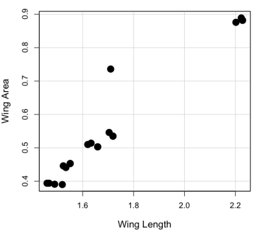
Figure 1. Scatterplot of Drosophila wing area by wing length

The R command for correlation is simply cor(x,y). This gives the “pearson” product moment correlation, the default. To specify other correlations, use method = “kendall”, or method = “spearman” (See Chapter 16.4).

Question. What are the Pearson, Spearman, and Kendall’s tau estimates for the correlation between fly Wing Length and Wing Area?

At the R prompt, type

cor(Length,Area) 
[1] 0.9693334 
cor(Length,Area, method="kendall") 
[1] 0.8248008 
cor(Length,Area, method="spearman") 
[1] 0.9558658

Note that we entered Length first. On your own, confirm that the order of entry does not change the correlation estimate. To both estimate test the significance of the correlation between Wing Area and Wing Length, at the R prompt type

cor.test(Area, Length, alternative="two.sided", method="pearson")

R returns with

Pearson's product-moment correlation 

data: Area and Length 

t = 16.735, df = 18, p-value = 2.038e-12>
alternative hypothesis: true correlation is not equal to 0
95 percent confidence interval:
0.9225336 0.9880360
sample estimates:
   cor
0.9693334

Alternatively, to calculate and test the correlation, use R Commander, Rcmdr: Statistics → Summaries→ Correlation test

R’s cor.test uses Fisher’s z transformation; note if we instead use the approximate calculation instead how poor the approximation works in this example. The estimated correlation was 0.97, thus the approximate standard error was 0.058. The confidence interval (t-distribution, alpha=0.05/2 and 18 degrees of freedom) was between 0.848 and 1.091, which is greater than the z transform result and returns an out-of-bounds upper limit.

Alternative packages to base R provide more flexibility and access to additional approaches to significance testing of correlations (Goertzen and Cribbie 2010). For example, z_cor_test() from the TOSTER package.

z_cor_test(Area, Length)

Pearson's product-moment correlation
data:  Area and Length
z = 8.5808, N = 20, p-value < 2.2e-16
alternative hypothesis: true correlation is not equal to 0
95 percent confidence interval:
0.9225336 0.9880360
sample estimates:
      cor
0.9693334

To confirm, check the critical value for z = 8.5808, two-tailed, with

> 2*pnorm(c(8.5808), mean=0, sd=1, lower.tail=FALSE)
[1] 9.421557e-18

Note the difference is that Fisher’s z is used for hypothesis testing; cor.test and z_cor_test return same confidence intervals.

and by bootstrap resampling (see Chapter 19.2),

boot_cor_test(Area, Length)

Bootstrapped Pearson's product-moment correlation

data: Area and Length
N = 20, p-value < 2.2e-16
alternative hypothesis: true correlation is not equal to 0
95 percent confidence interval:
0.8854133 0.9984744
sample estimates:
cor
0.9693334

The z-transform confidence interval would be preferred over the bootstrap confidence interval because it is narrower.

Assumptions of the product-moment correlation

Interestingly enough, there are no assumptions for estimating a statistic. You can always calculate an estimate, although of course, this does not mean that you have selected the best calculation to describe the phenomenon in question, it just means that assumptions are not applicable for estimation. Whether it is the sample mean or the correlation, it is important to appreciate that, look, you can always calculate it, even if it is not appropriate!

Statistical assumptions and those technical hypotheses we evaluate apply to statistical inference — being able to correctly interpret a test of statistical significance for a correlation estimate depends on how well assumptions are met. The most important assumption for a null hypothesis test of correlation is that samples were obtained from a “bivariate normal distribution.” It is generally sufficient to just test normality of the variables one at a time (univariate normality), but the student should be aware that testing the bivariate normality assumption can be done directly (e.g., Doornick and Hansen 2008).

Testing two independent correlations

Extending from a null hypothesis of the correlation is equal to zero to the correlation equals a particular value should not be a stretch for you. For example, since we use the t-test to evaluate the null hypothesis that the correlation is equal to zero, you should be able to make the connection that, like the two sample t-test, we can extend the test of correlation to any value. However, using the t-test without considering the need to stabilize the variance.

When two correlations come from independent samples, we can test whether or not the two correlations are equal. Rather than use the t-test, however, we use a modification of Fisher’s Z transformation. Calculate z for each correlation separately, then use the following equation to obtain Z. We then look up Z from our table of standard normal distribution (Appendix 20.1, or better — use the normal distribution functions in Rcmdr) and we can obtain the p-value of the test of the hypothesis that the two correlations are equal.

$\begin{align*} Z= \frac{z_{1}-z_{2}}{\sqrt{\frac{1}{n_{1}-3}+\frac{1}{n_{2}-3}}} \end{align*}$

Example. Two independent correlations are r1 = 0.2 and r2 = 0.34. Sample sizes for group 1 was 14 and for group 2 was 21. Test the hypothesis that the two correlations are equal. Using R as a calculator, here’s what we might write in the R script window and the resulting output. It doesn’t matter which correlation we set as r1 or r2, so I prefer to calculate the absolute value of Z and then get the probability from the normal table for values greater or equal to |Z| (i.e., the upper tail).

z1 = atanh(0.2)
z2 = atanh(0.34)
n1 = 14
n2 = 21
Z = abs((z1-z2)/sqrt((1/(n1-3))+(1/(n2-3))))
Z = 0.3954983

From the normal distribution table we get a p-value of 0.3462 for the upper tail. Because this p-value is not less than our typical Type I error rate of 0.05, we conclude that the two correlations are not in fact significantly different.

Rcmdr: Distributions → Continuous distributions → Normal distribution → Normal probabilities…

pnorm(c(0.3954983), mean=0, sd=1, lower.tail=FALSE)

R returns

[1] 0.3462376

To make this two-tailed, of course all we have to do is multiple the one-tailed p-value by two, in this case two-tailed p-value = 0.69247.

Write a function in R

There’s nothing wrong with running the calculations as written. But R allows users to write their own functions. Here’s one possible function we could write to test two independent correlations. Write the R function in the script window.

test2Corr = function(r1,r2,n1,n2) {
z1=atanh(r1); z2=atanh(r2)
Z = abs((z1-z2)/sqrt((1/(n1-3))+(1/(n2-3))))
pnorm(c(Z), mean=0, sd=1, lower.tail=FALSE)
}

After submitting the function, we then invoke the function by typing at the R prompt

p = test2Corr(0.2,0.34,14,21); p

Again, R returns the one-tailed p-value

[1] 0.3462376

Unsurprisingly, these simple functions are often available in an R package. In this case, the psych package provides a function called r.test() which will accommodate the test of the equality hypothesis of two independent correlations. Assuming that the psych package has been installed, at the R prompt we type

require(psych)
r.test(14,.2,.34,n2=21,twotailed=TRUE)

And R returns

Correlation tests
Call:r.test(n = 14, r12 = 0.20, r34 = 0.34, n2 = 21, twotailed = TRUE)
Test of difference between two independent correlations
z value 0.4 with probability 0.69

Questions

True of False. It is relatively easy to move from the estimation of one correlation between two continuous variables, to the estimation of multiple pairwise (“2 at a time”) correlations among many variables. For k = the number of variables, there are k(k-1)/2 unique correlations. However, one should be concerned about the multiple comparisons problem as introduced in ANOVA when one tests for the statistical significance of many correlations.
True or False. Generally, the null hypothesis of a test of a correlation is Ho: r = 0, although in practice, one could test a null of r = any value.
Return to the fly wing example. What was the estimate of the value of the product moment correlation? The Spearman Rank correlation? The Kendall’s tau?
OK, you have three correlation estimates for test of the same null hypothesis, i.e., correlation between Length and Area is zero. Which estimate is the best estimate?
Apply the Fisher z transformation to the estimated correlation, what did you get?
For the fly wing example, what were the degrees of freedom?
For the fly wing example, calculate the approximate standard error of the product moment correlation.
Return one last time to the fly wing example. What was the value of the lower limit of the 95% confidence interval for the estimate of the product moment correlation? And the value of the upper limit?
Assume that another group of students (n = 15) made measurements on fly wings and the correlation was 0.86. Is the difference between the two correlations for the two groups of students equal? Obtain the probability using the Z calculation and R (Chapter 6.7) or the normal table.