10.3 – Paired t-test
Introduction
Good experiments include controls. Interested in a new treatment for weight loss? Define a control group to compare the weight loss by a group using the new product. In many cases, the best control is the individual.
Consider now a basic experimental design, the randomized crossover trial (Fig. 1), introduced in Chapter 2.4.
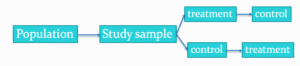
Figure 1. A two group Randomized Crossover Trial.
Subjects randomly selected from population of interest, then again once recruited into one of two treatment arms: arm 1, subjects first receive the experimental treatment, then some time later the subjects receive the control treatment; arm 2, subjects first receive the control treatment, then some time later the subjects receive the experimental treatment. Note the difference between this paired or repeated measures design and the independent sample design (see Chapter 10.1). Repeated measures designs have many advantages; we discuss them further in Chapter 14.6. At the start, repeated measures designs have greater statistical power compared to cross-sectional (independent) sample designs.
Many experiments are designed so that subjects receive all treatments and responses are gauged against the initial values recorded on the subjects. Repeated measures statistical tests, like the paired t-test, are needed however to analyze the data. These types of statistical procedures are similar to the two sample independent t-test that we discussed earlier.
However, there is an important difference between these two types of statistical procedures. For the two independent sample t-test the samples are unpaired: we observed one variable on some individuals assigned to two different groups. These groups might be
- Two locations where we measure plants or animals
- A treatment (or experimental) group with a control group.
- Expression of cytokeratin genes (e.g., ΔΔCT, fold-change) from breast cancer patients compared to healthy donor subjects (Andergassen et al 2016).
The point is that samples in one group are not the same samples in the second group.
In the paired t-test we have two groups but the observations in these two groups are paired. Paired means that there is some relationship between one observation in the first sample and one observation in the second sample (every observation in one sample must be paired with one observation in another sample).
For example, weight change in humans before and after a change in diet could be performed as a paired analysis. Each subject’s weight before the diet was “paired” with the same subject’s weight after the diet.
Another example comes from genetics. Siblings or Monozygotic twins or clones, strains or varieties of plants or animals can be Paired in an experiment.
- You can give one of the twins a particular diet, or the plant or animal clones or strains can be raised in a particular environment (nutrient)
- The other twin or plant or animal clone or variety can serve as a type of control by providing a normal diet or normal environment.
Another example is a study of environmental pollution on cancer rates in many different communities.
- The researchers selects pairs of communities with similar characteristics for many socioeconomic factors.
- Each pair of communities differed with respect to the proximity to a known source of pollution: one of the pair was close to a source of pollution and one of the pair was far from a source of pollution.
The purpose of pairing in this example is to attempt to “control” for all the socioeconomic factors that might contribute to cancer but they did not want to directly measure. These other factors should be similar for each member of the pair.
Example: How repeatable is human running performance?
The subheading is misleading — we leave “repeatability” or, do individuals perform consistently to another time (see Chapter 12.3 – Fixed effects, random effects, and agreement). Here, we focus on a different question — we test whether mean performance differs across repeated trials. This may seem a subtle difference, but consistency asks the question if performance, whether it is answering questions on an exam or running times for a race, is stable across trials. Testing the means of first and second trials asks a different question: we test for a trend in performance, which may reflect learning.
Here’s an example in which a measure was taken twice for the same individuals. The data are running speed or pace during 5K race held annually on Oahu for a selected sample of female runners with repeat race times (20 – 29 years old). The race was run annually on Oahu, and the data reported are the pace for the first race and the second race, which occurred a year later (Jamba Juice – Banana Man Chase, Ala Moana Beach Park, data extracted from source, https://timelinehawaii.com).
Table 1. 5K pace times (kph) for 15 women (20 – 29 years)
| ID | First race | Second race |
|---|---|---|
| 1 | 15.28 | 15.61 |
| 2 | 11.22 | 11.19 |
| 3 | 8.80 | 9.14 |
| 4 | 8.88 | 5.46 |
| 5 | 9.81 | 10.50 |
| 6 | 6.12 | 5.69 |
| 7 | 8.31 | 8.71 |
| 8 | 6.26 | 7.42 |
| 9 | 17.16 | 16.41 |
| 10 | 16.23 | 15.82 |
| 11 | 5.90 | 7.12 |
| 12 | 8.31 | 10.48 |
| 13 | 5.93 | 8.64 |
| 14 | 10.54 | 5.99 |
| 15 | 9.53 | 8.69 |
Note 1: We’ll return to this data set in Chapter 15.3
Load the data into R as an unstacked data set. Data available at end of this page or click here.
Begin with description and exploration of the data. Start with histograms to get a sense of the sample distributions (hint: we’re looking to see if the data looks like it could come from a normal distribution, see Chapter 13.3 Assumptions) (Fig 2).
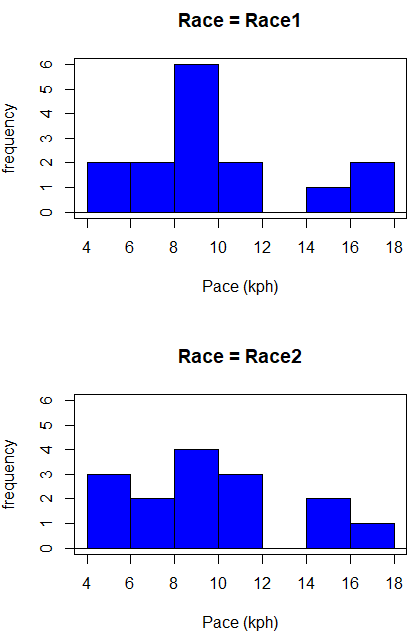
Figure 2. Histograms shows the distribution of 5K running times of 15 women who ran the race twice.
R code (stacked data set, then used defaults R Commander to make the histogram, then modified the code and submitted modified code to make Fig. 1)
with(stackExCh10.3, Hist(obs, groups=Race, scale="frequency", breaks="Sturges", col="blue",
xlab="Time (min)", ylab="Frequency")))
Conclusion? The histograms don’t look normally distributed so we keep this in mind as we proceed. (See Chapter 13 – Assumptions of parametric tests for additional information about assumptions.)
A box plot comparing the first and second pace times (Fig 3).
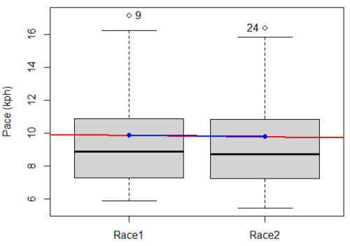
Figure 3. Box plot of race speed (kph) for 15 women 5K in two successive years.
I added a trend line (linear regression, see Chapter 17, red line) and connected the averages (blue line) for visual emphasis — no differences between the means — but note that one wouldn’t do this as part of an analysis (see Chapter 4 discussion).
R code for Fig. 2
Boxplot(obs~Race, data=stackExCh10.3, id=list(method="y"), xlab="", ylab="Pace (kph)") #boxplot was made in Rcmdr
abline(lm(obs ~ as.numeric(Race), data=stackExCh10.3), col="red", lwd=2)
means <- tapply(obs, Race, mean)
points(1:2, means, pch=7, col="blue")
lines(1:2, means, col="blue", lwd=2)
The box plot works to show the median difference, but loses the paired information. A nice package called PairedData has several functions that work well with paired data, for example a profile plot (Fig 4). A profile plot is useful for showing an association between paired data.
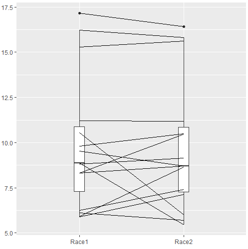
Figure 4. Profile plot, PairedData package.
R commands for Figure 4.
require(PairedData)
attach(example.ch10.3) # remember to attach dataframe so you don't have to call variables like example.ch10.3$Race1
races <- paired(Race1, Race2)
plot(races, type = "profile")
Paired t-test calculation
The paired t-test is a straight-forward extension of the independent sample t-test; the key concept is that the two samples are no longer independent, they are paired. Thus, instead of mean of group 1 minus mean of group two, we test the differences between sample 1 and sample 2 for each paired observation.

- Compute the differences between the Paired Samples (as in tables above)
- Calculate the MEAN difference score,
 : in the previous example = -0.094 kmh
 - Calculate the degrees of freedom df = # pairs – 1 = n – 1, where n is the number of pairs
- Calculate the standard error of the mean of d.

where

- Calculate the test statistic for paired data

- Compare to the Critical Value in Table C. 4 (Appendix Table 2)
- Find the Critical Value = t α (2), df
Try as difference instead of paired
Before you answer, take a look at the box plot of the mean difference between the repeat measures of 5K pace for the 15 women (Fig 5).
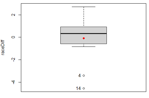
Figure 5. Box plot of differences, Red dotted lines shows the null hypothesis.
Note 2: Figure 5 is appropriate for diagnostics, but not for publication, per our discussions in Chapter 4.
Create a new variable, raceDiff, equal to Race2 minus Race1. Then, use the one sample T-test on raceDiff. I’ll leave you to complete the work (Question 2).
R code
t.test(Race1, Race2, paired = TRUE, alternative = "two.sided")
R output
Paired t-test

data: Race.1 and Race.2
t = 0.19389, df = 14, p-value = 0.849
alternative hypothesis: true difference in means is not equal to 0
95 percent confidence interval:
-0.9491017 1.1377521
sample estimates:
mean of the differences
0.09432517
Rcmdr, paired t-test
Rcmdr: Statistics → Means → Paired t-test…
Note: your two groups must be in two different columns (unstacked!) to run this version of the test.
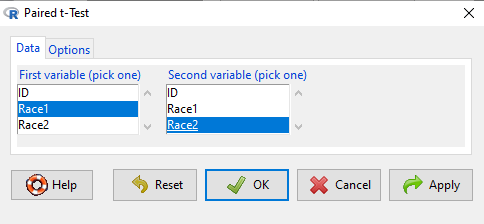
Figure 6. R Commander Paired t-test menu, Rcmdr version 2.7.
After selecting the variables, set null hypothesis after clicking on Options tab (Fig 6).
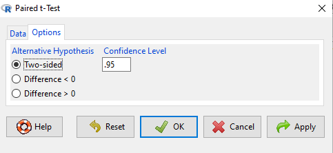
Figure 7. R Commander Paired t-Test options, select null hypothesis.
Click OK to proceed. Results will be the same as the output listed above.
the following text needs to be updated
Interpret the results.
So, what can we conclude about the null hypothesis? Interpret the 95% CI, the T-test statistic, and the P-value.
Do not ignore sample dependence
What if we ignored the repeated measures design and treated the first and second races as independent? The important concept here is to ask, what would have happened if we had done a two independent sample t-test instead?
Let’s run the analysis again, this time incorrectly using the independent sample t-test. We need to manipulate the data set before we do.
Manage your data: Stack the data
This is a good time to share how to Stack data in R. If you look at our active data set, the results of the two trials are in two different columns. In order to run the independent sample t-test we need the data in one column (with a label column).
stackExCh10.3 <- stack(example.ch10.3[, c("Race1","Race2")])
names(stackExCh10.3) <- c("obs", "Race")
Rcmdr: Data → Active data set → Stack variables in data set…
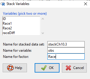
Figure 8. R Commander: Stack worksheet. Select the two variables, Race1 and Race2.
I entered values for name of the new data set, the new variable, and the name for the factor (label) column.
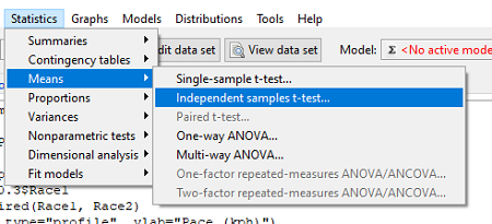
Figure 9. R Commander, select independent sample t-Test …
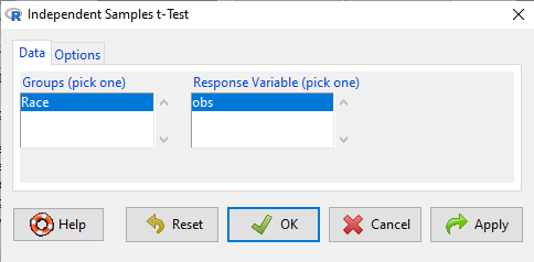
Figure 10. R commander, independent sample t test menu.
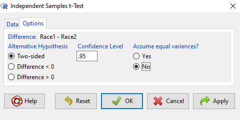
Figure 11. R Commander, select options for independent sample t-Test (assume equal variance).
Here are the results of the independent sample t-test from R.
t.test(obs~Race, alternative='two.sided', conf.level=.95, var.equal=TRUE, + data=stackCh10.3)

Two Sample t-test
data: obs by Race
t = 0.070645, df = 28, p-value = 0.9442
alternative hypothesis: true difference in means is not equal to 0
95 percent confidence interval:
 -2.640719 2.829369
sample estimates:
mean in group Race1 mean in group Race2
 9.886342 9.792017
End R output
In this case, we would have reached the same general conclusion, but the p-values are different. The p-value from the paired t-test was about 0.85 whereas the p-value from the independent sample t-test was higher, nearly 0.95, suggesting little difference between the two trials.
While the general conclusion holds, this time, that there were no statistically significant difference between the means for first and second trials. However, it won’t always work out that way. And besides, if you treated the paired data as independent, you’ve clearly violated one of the assumptions of the test.
Take a look at the degrees of freedom for the two analyses. By ignoring the pairing of samples we gain twice the number of degrees of freedom … that can’t both be right. The way to distinguish between the two is to go back to the experimental units.
Question: What are the sampling units in the case of repeat measures on individuals: the individuals themselves? the pairs of burst speed trials? something else?
it is important to note that the paired t-test is still the best for this situation because it accurately reflects the experiment — individuals were measured twice, therefore the two groups (trial 1 and trial 2) are not independent! Thus, the p-value from the paired t-test correctly reflect our best analyses of the test of the null hypothesis because the correct degrees of freedom were 14 and not 28.
In the case of the independent sample t-test we necessarily make the assumption that the two groups are independent — that is, that they are measured on different sampling units (e.g., different individuals or subjects). In statistical terms, that means that you assume that the correlation between trial results is equal to zero. By incorrectly choosing an independent sample test in these repeated measures cases, I would make two null hypotheses: (1) that the means are the same and (2) that the correlation between repeat measures is zero. The problem? The t-test only evaluates the first hypothesis (means).
Questions
- Refer to Figure 6 again and related data set. Were runners faster the second year or the first year running the 5k? What about the points labeled 4 and 14? What was the average difference between first and second races?
- Complete the test of the null hypothesis of no difference between race 1 and race 2 (
raceDiff) with the one sample t-test. Set up a table to compare the test statistic, df, and p-values for results from paired t test, one sample t-test, and independent sample t-test. How do these results compare? - I’ve called the observed value “pace,” but runners would know that pace is actually amount of time per kilometer, not the total time over 5k, which is what I called pace.
- Create a new variable and report average pace for Race1 and Race2.
- Redo the paired analysis, including box plot, on your new variable.
- What is the null hypothesis for your new variable?
- Summarize your results and add to the table you created for question 2.
- Redo the two plots in Figure 2 so that the two histograms are on the sample plot. Instructions and examples were provided in Chapter 4.2.
Quiz Chapter 10.3
Paired t-test
Data set
example.ch10.3 <- read.table(header=TRUE, text = "
ID Race1 Race2
1 15.28 15.61
2 11.22 11.19
3 8.80 9.14
4 8.88 5.46
5 9.81 10.50
6 6.12 5.69
7 8.31 8.71
8 6.26 7.42
9 17.16 16.41
10 16.23 15.82
11 5.90 7.12
12 8.31 10.48
13 5.93 8.64
14 10.54 5.99
15 9.53 8.69
")