18.3 – Logistic regression
Introduction
We briefly introduced logistic regression in the previous chapter on nonlinear regression. We expand our discussion of logistic regression here.
Logistic regression is a statistical method for modeling the dependence of a categorical (binomial) outcome variable on one or more categorical and continuous predictor variables (Bewick et al 2005).
The logistic function may be used to transform a sigmoidal curve to a more or less straight line while also changing the range of the data from binary (0 to 1) to infinity (-∞,+∞). For event with probability of occurring p, the logistic function is written as
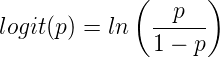
where ln refers to the natural logarithm.
This is an odds ratio. It represents the effect of the predictor variable on the chance that the event will occur.
The logistic regression model then very much resembles the same general linear models we have seen before.
![]()
In R and Rcmdr we use the glm() function to model the logistic function. Logistic regression is used to model a binary outcome variable. What is a binary outcome variable? It is categorical! Examples include: Living or Dead; Diabetes Yes or No; Coronary artery disease Yes or No. Male or Female. One of the categories could be scored 0, the other scored 1. For example, living might be 0 and dead might be scored as 1. (By the way, for a binomial variable, the mean for the variable is simply the number of experimental units with “1” divided by the total sample size.)
With the addition of a binary response variable, we are now really close to the Generalized Linear Model. Now we can handle statistical models in which our predictor variables are either categorical or ratio scale. All of the rules of crossed, balanced, nested, blocked designs still apply because our model is still of a linear form.
We write our generalized linear model

just to distinguish it from a general linear model with the ratio-scale Y as the response variable.
Think of the logistic regression as modeling a threshold of change between the 0 and the 1 value. In another way, think of all of the processes in nature in which there is a slow increase, followed by a rapid increase once a transition point is met, only to see the rate of change slow down again. Growth is like that (see Chapter 20.10 for related growth and related models). We start small, stay relatively small until birth, then as we reach our early teen years, a rapid change in growth (height, weight) is typically seed (well, not in my case … at least for the height). The curve I described is a logistic one (other models exist too). Where the linear regression function was used to minimize the squared residuals as the definition of the best fitting line, now we use the logistic as one possible way to describe or best fit this type of a curved relationship between an outcome and one or more predictor variables. We then set out to describe a model which captures when an event is unlikely to occur (the probability of dying is close to zero) AND to also describe when the event is highly likely to occur (the probability is close to one).
A simple way to view this is to think of time being the predictor (X) variable and risk of dying. If we’re talking about the lifetime of a mouse (lifespan typically about 18-36 months), then the risk of dying at one months is very low, and remains low through adulthood until the mouse begins the aging process. Here’s what the plot might look like, with the probability of dying at age X on the Y axis (probability = 0 to 1) (Fig 1).
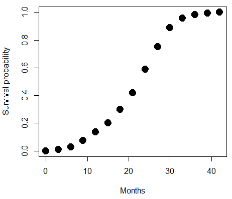
Figure 1. Lifespan of 1881 mice from 31 inbred strains (Data from Yuan et al [2012] available at https://phenome.jax.org/projects/Yuan2).
Note 1: I labeled Y axis labeled “Survival Probability”; “Inverse Survival Probability” would be more accurate.
We ask — of all the possible models we could draw — which model best fits the data? The curve fitting process is called the logistic regression. The sample data set is listed at end of this page (scroll down of click here). Create data.frame called yuan.
With some minor, but important differences, running the logistic regression is the same as what you have been doing so far for ANOVA and for linear regression. In Rcmdr, access the logistic regression function by calling the Generalized Linear Model (Fig 2).
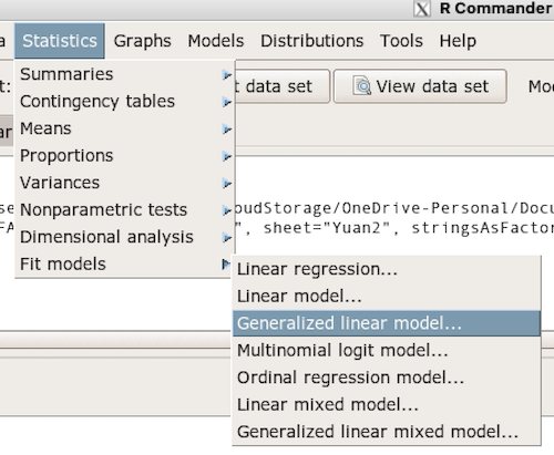
Figure 2. Access Generalized Linear Model via R Commander
R results
GLM.1 <- glm(cumFreq ~ Months, family=gaussian(identity), data=yuan)

> summary(GLM.1)

Call:
glm(formula = cumFreq ~ Months, family = gaussian(identity),
data = yuan)

Deviance Residuals:
     Min       1Q   Median      3Q     Max
-0.11070 -0.07799 -0.01728 0.06982 0.13345

Coefficients:
             Estimate Std. Error t value Pr(>|t|)
(Intercept) -0.132709   0.045757   -2.90 0.0124 *
Months       0.029605   0.001854   15.97 6.37e-10 ***
---
Signif. codes: 0 '***' 0.001 '**' 0.01 '*' 0.05 '.' 0.1 ' ' 1

(Dispersion parameter for gaussian family taken to be 0.008663679)

Null deviance: 2.32129 on 14 degrees of freedom
Residual deviance: 0.11263 on 13 degrees of freedom
AIC: -24.808

Number of Fisher Scoring iterations: 2
Rcmdr: Statistics → Fit models → Generalized linear model.
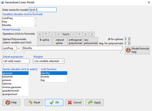
Figure 3. Screenshot Rcmdr GLM menu. For logistic on ratio-scale dependent variable, select gaussian family and identity link function.
Select the model as before. The box to the left accepts your binomial dependent variable; the box at right accepts your factors, your interactions, and your covariates. It permits you to inform R how to handle the factors: Crossed? Just enter the factors and follow each with a plus. If fully crossed, then the interactions may be specified with “:” to explicitly call for a two-way interaction between two (A:B) or a three-way interaction between three (A:B:C) variables. In the later case, if all of the two way interactions are of interest, simply typing A*B*C would have done it. If nested, then use %in% to specify the nesting factor.
R output
GLM.1 <- glm(cumFreq ~ Months, family=gaussian(identity), data=yuan)

summary(GLM.1)

Call:
glm(formula = cumFreq ~ Months, family = gaussian(identity),
data = yuan)

Deviance Residuals:
     Min       1Q   Median      3Q     Max
-0.11070 -0.07799 -0.01728 0.06982 0.13345

Coefficients:
               Estimate   Std. Error   t value   Pr(>|t|)
(Intercept)   -0.132709     0.045757   -2.90     0.0124 *
Months         0.029605     0.001854   15.97     6.37e-10 ***
---
Signif. codes: 0 '***' 0.001 '**' 0.01 '*' 0.05 '.' 0.1 ' ' 1

(Dispersion parameter for gaussian family taken to be 0.008663679)

Null deviance: 2.32129 on 14 degrees of freedom
Residual deviance: 0.11263 on 13 degrees of freedom
AIC: -24.808

Number of Fisher Scoring iterations: 2
Note 2: The %in% operator is an infix function used to determine if elements of a vector or object on the left-hand side are present within another vector or object on the right-hand side. Quietly, we introduced use of %in% in our code to subset data set in a BONUS problem.
Assessing fit of the logistic regression model
Some of the differences you will see with the logistic regression is the term “deviance.” deviance in statistics simply means compare one model to another and calculate some test statistic we’ll call “the deviance.” We then evaluate the size of the deviance like a chi-square goodness of fit. If the model fits the data poorly (residuals large relative to the predicted curve), then the deviance will be small and the probability will also be high — the model explains little of the data variation. On the other hand, if the deviance is large, then the probability will be small — the model explains the data, and the probability associated with the deviance will be small (significantly so? You guessed it! P < 0.05).
The Wald statistic

where n and β refers to any of the n coefficient from the logistic regression equation and SE refers to the standard error if the coefficient. The Wald test is used to test the statistical significance of the coefficients. It is distributed approximately as a chi-squared probability distribution with one degree of freedom. The Wald test is reasonable, but has been found to give values that are not possible for the parameter (eg, negative probability).
Likelihood ratio tests are generally preferred over the Wald test. For a coefficient, the likelihood test is written as
![]()
where L0 is the likelihood of the data when the coefficient is removed from the model (ie, set to zero value), whereas L1 is the likelihood of the data when the coefficient is the estimated value of the coefficient. It is also distributed approximately as a chi-squared probability distribution with one degree of freedom.
Nonlinear regression
Nonlinear regression, nls() function, may be a better choice. The following
attach(yuan)
logisticModel <-nls(cumFreq~DD/(1+exp(-(CC+bb*Months))), start=list(DD=1,CC=0.2,bb=.5),data=yuan,trace=TRUE)
summary(logisticModel)

Formula: yuan$cumFreq ~ DD/(1 + exp(-(CC + bb * yuan$Months)))

Parameters:
      Estimate   Std. Error    t value    Pr(>|t|)
DD    1.038504     0.014471      71.77    < 2e-16 ***
CC   -4.626982     0.175109     -26.42   5.29e-12 ***
bb    0.206899     0.008777      23.57   2.03e-11 ***
---
Signif. codes: 0 '***' 0.001 '**' 0.01 '*' 0.05 '.' 0.1 ' ' 1

Residual standard error: 0.01908 on 12 degrees of freedom

Number of iterations to convergence: 11
Achieved convergence tolerance: 0.000006909
Get fit statistics
AIC(logisticModel)
[1] -71.54679
Because AIC for the nonlinear model much smaller (more negative) than AIC for logistic model, we may be tempted to judge fit of the nonlinear regression as best. However, this comparison of models is not valid because the Y variables are different between the two models and the fit families are different. One option, evaluate fit of models by plots of residuals (see 17.7 – Regression model fit).
Questions
1. Write up three learning outcomes for this page. Hint: Point your favorite generative AI to this page and ask for help.
Quiz Chapter 18.3
Logistic regression
Data set this page
| Months | freq | cumFreq |
|---|---|---|
| 0 | 0 | 0 |
| 3 | 0.010633 | 0.010633 |
| 6 | 0.017012 | 0.027645 |
| 9 | 0.045189 | 0.072834 |
| 12 | 0.064327 | 0.137161 |
| 15 | 0.064859 | 0.20202 |
| 18 | 0.09782 | 0.299841 |
| 21 | 0.118554 | 0.418394 |
| 24 | 0.171186 | 0.58958 |
| 27 | 0.162148 | 0.751728 |
| 30 | 0.137161 | 0.888889 |
| 33 | 0.069644 | 0.958533 |
| 36 | 0.024455 | 0.982988 |
| 39 | 0.011696 | 0.994684 |
| 42 | 0.005316 | 1 |