20.10 – Growth equations and dose response calculations
Introduction
In biology, growth may refer to increase in cell number, change in size of an individual across development, or increase of number of individuals in a population over time. Nonlinear, time-series, several models proposed to fit growth data, including the Gompertz, logistic, and the von Bertalanffy. These models fit many S-shaped growth curves. These models are special cases of generalized linear models, also called Richard curves.
Growth example
This page describes how to use R to analyze growth curve data sets.
| Hours | Abs |
|---|---|
| 0.000 | 0.002207 |
| 0.274 | 0.010443 |
| 0.384 | 0.033688 |
| 0.658 | 0.063257 |
| 0.986 | 0.111848 |
| 1.260 | 0.249240 |
| 1.479 | 0.416236 |
| 1.699 | 0.515578 |
| 1.973 | 0.572632 |
| 2.137 | 0.589528 |
| 2.466 | 0.619091 |
| 2.795 | 0.608486 |
| 3.123 | 0.621136 |
| 3.671 | 0.616850 |
| 4.110 | 0.614689 |
| 4.548 | 0.614643 |
| 5.151 | 0.612465 |
| 5.534 | 0.606082 |
| 5.863 | 0.603933 |
| 6.521 | 0.595407 |
| 7.068 | 0.589006 |
| 7.671 | 0.578372 |
| 8.164 | 0.567749 |
| 8.877 | 0.559217 |
| 9.644 | 0.546451 |
| 10.466 | 0.537907 |
| 11.233 | 0.537826 |
| 11.890 | 0.529300 |
| 12.493 | 0.516551 |
| 13.205 | 0.505905 |
| 14.082 | 0.491013 |
Key to parameter estimates: y0 is the lag, mumax is the growth rate, and K is the asymptotic stationary growth phase. The spline function does not return an estimate for K.
R code
require(growthrates)
#Enter the data. Replace these example values with your own
#time variable (Hours)
Hours <- c(0.000, 0.274, 0.384, 0.658, 0.986, 1.260, 1.479, 1.699, 1.973, 2.137, 2.466, 2.795, 3.123, 3.671, 4.110, 4.548, 5.151, 5.534, 5.863, 6.521, 7.068, 7.671, 8.164, 8.877, 9.644, 10.466, 11.233, 11.890, 12.493, 13.205, 14.082)
#absorbance or concentration variable (Abs)
Abs <- c(0.002207, 0.010443, 0.033688, 0.063257, 0.111848, 0.249240, 0.416236, 0.515578, 0.572632, 0.589528, 0.619091, 0.608486, 0.621136, 0.616850, 0.614689, 0.614643, 0.612465, 0.606082, 0.603933, 0.595407, 0.589006, 0.578372, 0.567749, 0.559217, 0.546451, 0.537907, 0.537826, 0.529300, 0.516551, 0.505905, 0.491013)
#Make a dataframe and check the data; If error, then check that variables have equal numbers of entries
Yeast <- data.frame(Hours,Abs); Yeast
#Obtain growth parameters from fit of a parametric growth model
#First, try some reasonable starting values
p <- c(y0 = 0.001, mumax = 0.5, K = 0.6)
model.par <- fit_growthmodel(FUN = grow_logistic, p = p, Hours, Abs, method=c("L-BFGS-B"))
summary(model.par)
coef(model.par)
#Obtain growth parameters from fit of a nonparametric smoothing spline
model.npar <- fit_spline(Hours,Abs)
summary(model.npar)
coef(spline.md)
#Make plots
par(mfrow = c(2, 1))
plot(Yeast, ylim=c(0,1), cex=1.5,pch=16, main="Parametric Nonlinear Growth Model", xlab="Hours", ylab="Abs")
lines(model.par, col="blue", lwd=2)
plot(model.npar, ylim=c(0,1), lwd=2, main="Nonparametric Spline Fit", xlab="Hours", ylab="Abs")
Results from example code
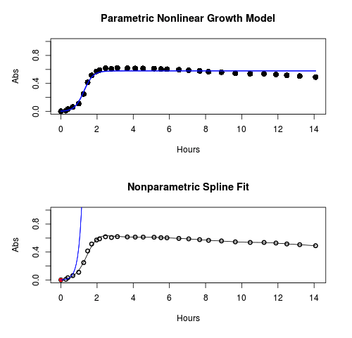
Figure 1. Top: Parametric Nonlinear Growth Model; Bottom: Nonparametric Spline Fit
LD50
In toxicology, the dose of a pathogen, radiation, or toxin required to kill half the members of a tested population of animals or cells is called the lethal dose, 50%, or LD50. This measure is also known as the lethal concentration, LC50, or properly after a specified test duration, the LCt50 indicating the lethal concentration and time of exposure. LD50 figures are frequently used as a general indicator of a substance’s acute toxicity. A lower LD50 is indicative of increased toxicity.
The point at which 50% response of studied organisms to range of doses of a substance (e.g., agonist, antagonist, inhibitor, etc.) to any response, from change in behavior or life history characteristics up to and including death can be described by the methods described in this chapter. The procedures outlined below assume that there is but one inflection point, i.e., an “s-shaped” curve, either up or down; if there are more than one inflection points, then the logistic equations described will not fit the data well and other choices need to be made (see Di Veroli et al 2015). We will use the drc package (Ritz et al 2015).
Example
First we’ll work through use of R. We’ll follow up with how to use Solver in Microsoft Excel.
After starting R, load the drc library.
library(drc)
Consider some hypothetical 24-hour survival data for yeast exposed to salt solutions. Let resp equal the variable for frequency of survival (e.g., calculated from OD660 readings) and NaCl equal the millimolar (mm) salt concentrations or doses.
At the R prompt type
resp <- c(1,1,1,.9,.7,.3,.4,.2,0,0,0)
NaCl=seq(0,1000,100)
#Confirm sequence was correctly created; alternatively, enter the values.
NaCl
[1] 0 100 200 300 400 500 600 700 800 900 1000
#Make a plot
plot(NaCl,resp,pch=19,cex=1.2,col="blue",xlab="NaCl [mm]",ylab="Survival frequency")
And here is the plot (Fig. 2).
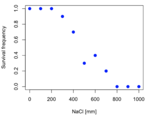
Figure 2. Hypothetical data set, survival of yeast in different salt concentrations.
Note the sigmoidal “S” shape — we’ll need an logistic equation to describe the relationship between survival of yeast and NaCl doses.
The equation for the four parameter logistic curve, also called the Hill-Slope model, is

where c is the parameter for the lower limit of the response, d is the parameter for the upper limit of the response, e is the relative EC50, the dose fitted half-way between the limits c and d, and b is the relative slope around the EC50. The slope, b, is also known as the Hill slope. Because this experiment included a dose of zero, a three parameter logistic curve would be appropriate. The equation simplifies to

EC50 from 4 parameter model
Let’s first make a data frame
dose <- data.frame(NaCl, resp)
Then call up a function, drm, from the drc library and specify the model as the four parameter logistic equation, specified as LL.4(). We follow with a call to the summary command to retrieve output from the drm function. Note that the four-parameter logistic equation
model.dose1 = drm(dose,fct=LL.4())
summary(model.dose1)
And here is the R output.
Model fitted: Log-logistic (ED50 as parameter) (4 parms)
Parameter estimates:
                   Estimate  Std. Error    t-value  p-value
b:(Intercept)      3.753415    1.074050   3.494636   0.0101
c:(Intercept)     -0.084487    0.127962  -0.660251   0.5302
d:(Intercept)      1.017592    0.052460  19.397441   0.0000
e:(Intercept)    492.645128   47.679765  10.332373   0.0000

Residual standard error:
0.0845254 (7 degrees of freedom)
The EC50, technically the LD50 because the data were for survival, is the value of e: 492.65 mM NaCl.
You should always plot the predicted line from your model against the real data and inspect the fit.
At the R prompt type
plot(model.dose1, log="",pch=19,cex=1.2,col="blue",xlab="NaCl [mm]",ylab="Survival frequency")
As long as the plot you made in earlier steps is still available, R will add the line specified in the lines command. Here is the plot with the predicted logistic line displayed (Fig. 3).
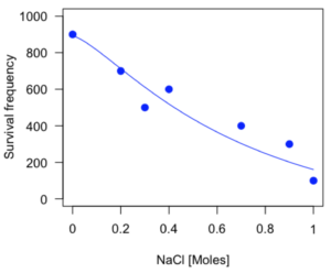
Figure 3. Logistic curve added to Figure 1 plot.
While there are additional steps we can take to decide is the fit of the logistic curve was good to the data, visual inspection suggests that indeed the curve fits the data reasonably well.
More work to do
Because the EC50 calculations are estimates, we should also obtain confidence intervals. The drc library provides a function called ED which will accomplish this. We can also ask what the survival was at 10% and 90% in addition to 50%, along with the confidence intervals for each.
At the R prompt type
ED(model.dose1,c(10,50,90), interval="delta")
And the output is shown below.
Estimated effective doses
(Delta method-based confidence interval(s))
     Estimate Std. Error   Lower   Upper
1:10  274.348     38.291 183.803  364.89
1:50  492.645     47.680 379.900  605.39
1:90  884.642    208.171 392.395 1376.89
Thus, the 95% confidence interval for the EC50 calculated from the four parameter logistic curve was between the lower limit of 379.9 and an upper limit of 605.39 mm NaCl.
EC50 from 3 parameter model
Looking at the summary output from the four parameter logistic function we see that the value for c was -0.085 and p-value was 0.53, which suggests that the lower limit was not statistically different from zero. We would expect this given that the experiment had included a control of zero mm added salt. Thus, we can explore by how much the EC50 estimate changes when the additional parameter c is no longer estimated by calculating a three parameter model with LL.3().
model.dose2 = drm(dose,fct=LL.3())
summary(model.dose2)
R output follows.
Model fitted: Log-logistic (ED50 as parameter) with lower limit at 0 (3 parms)
Parameter estimates:
               Estimate Std. Error   t-value p-value
b:(Intercept)   4.46194    0.76880   5.80378   4e-04
d:(Intercept)   1.00982    0.04866  20.75272   0e+00
e:(Intercept) 467.87842   25.24633  18.53253   0e+00
Residual standard error:
 0.08267671 (8 degrees of freedom)
The EC50 is the value of e: 467.88 mM NaCl.
How do the four and three parameter models compare? We can rephrase this as as statistical test of fit; which model fits the data better, a three parameter or a four parameter model?
At the R prompt type
anova(model.dose1, model.dose2)
The R output follows.
1st mode
fct:      LL.3()
2nd model
fct:      LL.4()
ANOVA table
          ModelDf      RSS Df F value p value
2nd model       8 0.054684
1st model       7 0.050012  1  0.6539  0.4453
Because the p-value is much greater than 5% we may conclude that the fit of the four parameter model was not significantly better than the fit of the three parameter model. Thus, based on our criteria we established in discussions of model fit in Chapter 16 – 18, we would conclude that the three parameter model is the preferred model.
The plot below now includes the fit of the four parameter model (red line) and the three parameter model (green line) to the data (Fig. 4).
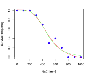
Figure 4. Four parameter (red) and three parameter (green) logistic models fitted to data.
The R command to make this addition to our active plot was
lines(dose,predict(model.dose2, data.frame(x=dose)),col="green")
We continue with our analysis of the three parameter model and produce the confidence intervals for the EC50 (modify the ED() statement above for model.dose2 in place of model.dose1).
Estimated effective doses
(Delta method-based confidence interval(s))
     Estimate Std. Error   Lower  Upper
1:10  285.937     33.154 209.483 362.39
1:50  467.878     25.246 409.660 526.10
1:90  765.589     63.026 620.251 910.93
Thus, the 95% confidence interval for the EC50 calculated from the three parameter logistic curve was between the lower limit of 409.7 and an upper limit of 526.1 mm NaCl. The difference between upper and lower limits was 116.4 mm NaCl, a smaller difference than the interval calculated for the 95% confidence intervals from the four parameter model (225.5 mm NaCl). This demonstrates the estimation trade-off: more parameters to estimate reduces the confidence in any one parameter estimate.
Additional notes of EC50 calculations
Care must be taken that the model fits the data well. What if we did not have observations throughout the range of the sigmoidal shape? We can explore this by taking a subset of the data.
dd = dose[1:6,]
Here, all values after dose 500 were dropped
dd
  resp dose
1  1.0    0
2  1.0  100
3  1.0  200
4  0.9  300
5  0.7  400
6  0.3  500
and the plot does not show an obvious sigmoidal shape (Fig. 5).
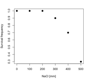
Figure 5. Plot of reduced data set.
We run the three parameter model again, this time on the subset of the data.
model.dosedd = drm(dd,fct=LL.3())
summary(model.dosedd)
Output from the results are
Model fitted: Log-logistic (ED50 as parameter) with lower limit at 0 (3 parms)
Parameter estimates:
                Estimate Std. Error    t-value p-value
b:(Intercept)   6.989842   0.760112   9.195801  0.0027
d:(Intercept)   0.993391   0.014793  67.153883  0.0000
e:(Intercept) 446.882542   5.905728  75.669344  0.0000
Residual standard error:
 0.02574154 (3 degrees of freedom)
Conclusion? The estimate is different, but only just so, 447 vs. 468 mm NaCl.
Thus, within reason, the drc function performs well for the calculation of EC50. Not all tools available to the student will do as well.
NLopt and nloptr
draft
Free open source library for nonlinear optimization.
Steven G. Johnson, The NLopt nonlinear-optimization package, http://github.com/stevengj/nlopt
https://cran.r-project.org/web/packages/nloptr/vignettes/nloptr.html
Alternatives to R
What about online tools? There are several online sites that will allow students to perform these kinds of calculations. Students familiar with MatLab know that it can be used to solve nonlinear equation problems. An open source alternative to MatLab is called GNU Octave, which can be installed on a personal computer or run online at http://octave-online.net. Students also may be aware of other sites, e.g., mycurvefit.com and IC50.tk.
Both of these free services performed well on the full dataset (results not shown), but fared poorly on the reduced subset: mycurvefit returned a value of 747.64 and IC50.tk returned an EC50 estimate of 103.6 (Michael Dohm, pers. obs.).
Simple inspection of the plotted values shows that these values are unreasonable.
EC50 calculations with Microsoft Excel
Most versions of Microsoft Excel include an add-in called Solver, which will permit mathematical modeling. The add-in is not installed as part of the default installation, but can be installed via the Options tab in the File menu for a local installation or via Insert for the Microsoft Office online version of Excel (you need a free Microsoft account). The following instructions are for a local installation of Microsoft Office 365 and were modified from information provided by sharpstatistics.co.uk.
After opening Excel, set up worksheet as follows. Note that in order to use my formulas your spreadsheet values need to be set up exactly as I describe.
- Dose values in column A, beginning with row 2
- Response values in column B, beginning with row 2
- In column F type
bin row 2,cin row 3,din row 4, andein row 5. - In cells G2 – G5, enter the starting values. For this example, I used b = 1, c = 0, d = 1, e = 400.
- For your own data you will have to explore use of different starting values.
- Enter headers in row 1.
- Column A
Dose - Column B
Response - Column C
Predicted - Column D
Squared difference - Column F
Constants
- Column A
- In cell C14 enter
sum squares - In cell D14 enter
=sum(D2:D12)
Here is an image of the worksheet (Fig. 6), with equations entered and values updated, but before Solver run.
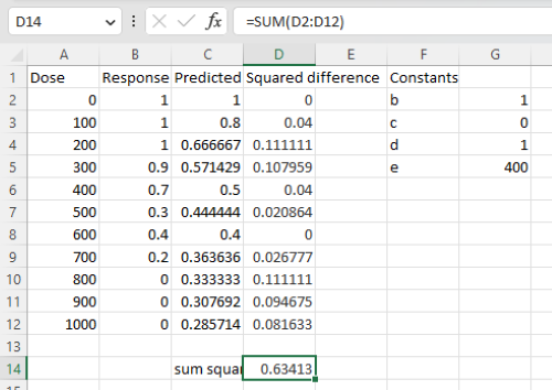
Figure 6. Screenshot Microsoft Excel worksheet containing our data set (col A & B), with formulas added and calculated. Starting values for constants in column G, rows 2 – 4.
Next, enter the functions.
- In cell C2 enter the four parameter logistic formula — type everything between the double quotes: “
=$G$3+(($G$4-$G$3)/(1+(A2/$G$5)^$G$2))“. Next, copy or drag the formula to cell C12 to complete the predictions.- Note: for a three parameter model, replace the above formula with “
=(($G$4)/(1+(A2/$G$5)^$G$2))“.
- Note: for a three parameter model, replace the above formula with “
- In cell D2 type everything between the double quotes: “
=(B2-C2)^2“. - Next, copy or drag the formula to cell
D12to complete the predictions. - Now you are ready to run solver to estimate the values for b, c, d, and e.
- Reminder: starting values must be in cells
G2:G5
- Reminder: starting values must be in cells
- Select cell
D14and start solver by clicking on Data and looking to the right in the ribbon.
Solver is not normally installed as part of the default installation of Microsoft Excel 365. If the add-in has been installed you will see Solver in the Analyze box (Fig. 7).
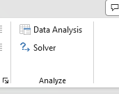
Figure 7. Screenshot Microsoft Excel, Solver add-in available.
If Solver is not installed, go to File → Options → Add-ins (Fig. 8).
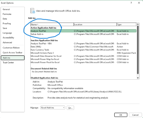
Figure 8. Screenshot Microsoft Excel, Solver add-in available and ready for use.
Go to Microsoft support for assistance with add-ins.
With the spreadsheet completed and Solver available, click on Solver in the ribbon (Fig. 7) to begin. The screen shot from the first screen of Solver is shown below (Fig. 9).
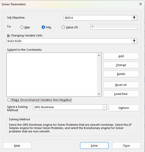
Figure 9. Screenshot Microsoft Excel solver menu.
Setup Solver
- Set Objective, enter the absolute cell reference to the sum squares value, \
$D$14 - Set To: Min.
- For By Changing Variable Cells, enter the range of cells for the four parameters, $G$2:$G$5
- Uncheck the box by “Make Unconstrained Variables Non-Negative.”
- Where constraints refers to any system of equalities or inequalities equations imposed on the algorithm.
- Select a Solving method, choose “GRG Nonlinear,” the nonlinear programming solver option (not shown in Fig. 7, select by clicking on the down arrow).
- Click Solve button to proceed.
GRG Nonlinear is one of many optimization methods. In this case we calculate the minimum of the sum of squares — the difference between observed and predicted values from the logistic equation — given the range of observed values. GRG stands for Generalized Reduced Gradient and finds the local optima — in this case the minimum or valley — without any imposed constraints. See solver.com for additional discussion of this algorithm.
If all goes well, this next screen (Fig. 10) will appear which shows the message, “Solver has converged to the current solution. All constraints are satisfied.”
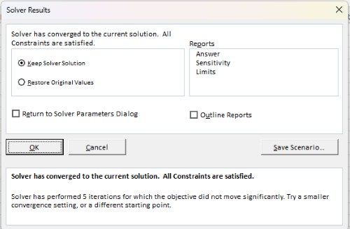
Figure 10. Screenshot solver completed run.
Click OK and note that the values of the parameters have been updated (Table 1).
Table 1. Four parameter logistic model, results from Solver
| Constant | Starting values | Values after solver |
| b | 1 | 3.723008382 |
| c | 0 | -0.088865487 |
| d | 1 | 1.017964505 |
| e | 400 | 493.9703594 |
Note the values obtained by Solver are virtually identical to the values obtained in the drc R package. The differences are probably because of the solver algorithm.
More interestingly, how did Solver do on the subset data set? Here are the results from a three parameter logistic model (Table 2).
Table 2. Three parameter logistic model, results from Solver
| Constant | Starting values | Full dataset, Solver results |
Subset, Solver results |
| b | 1 | 3.723008382 | 6.989855948 |
| d | 1 | 1.017964505 | 0.993391264 |
| e | 400 | 493.9703594 | 446.8819282 |
The results are again very close to results from the drc R package.
Thus, we would conclude that Solver and Microsoft Excel would be a reasonable choice for EC50 calculations, and much better than IC50.tk and mycurvefit.com. The advantages of R over Microsoft Excel is that the model building is more straightforward than entering formulas in the cell reference format required by Excel.
Questions
[pending]
References and suggested readings
Beck B, Chen YF, Dere W, et al. Assay Operations for SAR Support. 2012 May 1 [Updated 2012 Oct 1]. In: Sittampalam GS, Coussens NP, Nelson H, et al., editors. Assay Guidance Manual [Internet]. Bethesda (MD): Eli Lilly & Company and the National Center for Advancing Translational Sciences; 2004-. Available from: www.ncbi.nlm.nih.gov/books/NBK91994/
Di Veroli G. Y., Fornari C., Goldlust I., Mills G., Koh S. B., Bramhall J. L., Richards, F. M., Jodrell D. I. (2015) An automated fitting procedure and software for dose-response curves with multiphasic features. Scientific Reports 5: 14701.
Ritz, C., Baty, F., Streibig, J. C., Gerhard, D. (2015) Dose-Response Analysis Using R PLOS ONE, 10(12), e0146021
Tjørve, K. M., & Tjørve, E. (2017). The use of Gompertz models in growth analyses, and new Gompertz-model approach: An addition to the Unified-Richards family. PloS one, 12(6), e0178691.
Chapter 20 contents
- Additional topics
- Area under the curve
- Peak detection
- Baseline correction
- Surveys
- Time series
- Dimensional analysis
- Estimating population size
- Diversity indexes
- Survival analysis
- Growth equations and dose response calculations
- Plot a Newick tree
- Phylogenetically independent contrasts
- How to get the distances from a distance tree
- Binary classification
- Meta-analysis
/MD