14.3 – Fixed effects, Random effects
Introduction
With few exceptions (eg, repeatability and intraclass correlation calculations, Chapter 12.3), we have been discussing the Model I ANOVA or fixed-effects ANOVA– fixed implies that we select the levels for the factor. It may not be obvious — in hindsight it is — but levels may also be randomly selected, eg, nature provides the levels. Thus, levels are random and the model is a random-effects ANOVA. Beginning with our discussions of ANOVA, it becomes increasingly important to incorporate concept of models in statistics. As you have been working in R and Rcmdr with the lm() function, you have been forced to address the statistical model concept — you enter the response variable then type in both factors and create a term for the interaction.
We’ve just completed an experiment in which the response (cholesterol levels) of 36 individuals, from one of three drug treatments (placebo, Drug A, Drug B), given one of 3 types of diets (low, medium, or high carbohydrate), was observed. Thus, we say that the specific treatments of drug and diet contribute to variation in cholesterol levels. More formally, we say that the observed response of the kth individual (Yijk) is equal to the overall mean (m) plus the added effect of Drug (a) plus the added effect of Diet (b) plus the interaction between Diet and Population (ab) plus unidentified sources of variation generally called error (e). In symbols, we write

where i is the number of levels of the first factor (in our example, Diet had 2 levels, so i = A or i = B), j is the number of levels of the second factor (in our example, Population had 2 levels, so j = 1, or j = 2), and k is the total number of observations in the experiment (12 in our example, so k = 1, 2, …, 11, 12). Thus, we can think of each term “adding up” to give us the observed value.
Although it is a bit confusing at first, these equations help us understand how the experiment was conducted and therefore how to analyze and interpret the results.
Model I, Model II & Model III ANOVA
Statisticians recognize that how levels of the factors were selected for an experiment impact conclusions from ANOVAs. The key: whether or not the levels of the factor were selected (1) randomly from all possible levels of the factor or (2) specifically selected by the experimenters. We introduced the concepts of fixed and random effects in Chapter 12.3. For one-way ANOVA, the distinction between fixed and random effects influences the interpretation, but not the calculation of the ANOVA components. For two or more treatment factors, both the interpretations and the calculations of ANOVA components are affected.
There are two general types of Factors that we can choose to employ in an ANOVA: Fixed Model ANOVA and Random Model ANOVA. Where two or more factors apply, by far the most common model in experimental sciences is a combination of fixed and random, so we need to add a third general type, the Mixed Model ANOVA design.
Fixed Factors. Where the levels of the factor are selected by us. In this case we would only be interested in the response of the individuals that are given those specific treatments.
Medicine – for example, where we choose a treatment given to patients with a history of coronary heart disease; compare outcomes of patients given a statin (drug used to lower serum cholesterol) drug versus a placebo. (Note that this is the same study we discussed in our lecture on about risk analysis).
Ecotoxicology – for example, compare growth rates and deformities of tadpole frogs given Aldicarb, Atrazine (both estrogen-mimicking pesticides), or a control (ie, no pesticides). If you’re interested in these topics, here’s a link to the EPA’s web site, listing pesticide sales and use in the United States. Here’s a link to a NIH National Institute of Environmental Sciences, with a nice description of estrogen mimicking pesticides.
Agriculture & Genetics – for example, monitor growth of a particular hybrid corn available from three different manufacturers. See an example of Wisconsin corn hybrid studies.
In each of these examples we might be interested in those specific treatments and no other treatments.
HO: No difference in the means among the levels of the Factor
HA: Some difference in the means among these specific levels of the Factor; the specific levels of this factor affects the response variable.
This is an example of a Model I ANOVA, also called a “fixed effects” model ANOVA.
Random Factors. We still only use a relatively few number of different levels of a particular factor. However, in this case we are interested in many different levels of the factor — we want to generalize beyond our sample. The levels that we use would be a “sample” of all possible levels that we would be interested in.
Medicine – for example, where we randomly choose a treatment level given to patients; four concentrations of a drug and a placebo. Since concentration is a ratio scale data type, concentration can range from 0 (the placebo) to 100%.
Ecotoxicology – for example, release different concentrations or mixtures of air plus components of air pollution to chambers, record the response of plants or animals.
Agriculture & Genetics – for example, grow three different varieties of a plant in three different soils or different genetic strains of animals on three different diets. In these cases, factor levels are random because we are drawing from a large pool of possible levels: genetic varieties or strains — we selected three, but it’s rare that were are specifically interested in the three chosen. More often, we want to make generalizations and the three were somehow representative (we hope) of genetic variation in the species of interest.
In each of these examples, we write the null hypothesis to reflect that the particular levels are only of interest in so far as they can be used to generalize back to the population.
HO: No difference in the variation between groups.
HA: Some difference in the variation among these groups.
This is an example of a Model II ANOVA, also called a “random effects” model ANOVA. Note that we specify the hypothesis in terms of variation, not of the means.
Your two-way ANOVA could be Model I, Model II, or it could be mixed, with one factor fixed, the other random (this later model is called a Model III, or “mixed model” ANOVA).
For the most part, the distinction between whether you have fixed or random effects is clear, but whether we use fixed or random or combinations, this design decision has consequences for testing.
The decision does not affect the Sources of Variation for the different Models. Last time, we showed the tests for a Model I ANOVA (the “fixed effects model”).
For Random Effects or Mixed Effects, we only change how we determine the statistical significance of the Factors. Here’s a summary of how the experimental design changes the calculation of the F-test statistic for the Factors.
Table 1. Calculation of F
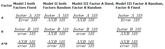
The Critical Value for each of the different F values will be obtained by simply finding the degrees of freedom for the numerator and denominator SS. This was discussed and can be found sources of variation in 2-way ANOVA lecture.
From the formulas, we can see that the major difference is that sometimes the Factor MS is divided by the error MS and sometimes it is divided by the interaction MS.
If the interaction term is NOT statistically significant, then the Interaction MS (mean square) estimates the Error MS. In other words, if the interaction term is not statistically significant it will be similar in magnitude as the Error MS. In this case there will be no large difference in the computed outcomes if the Factor A or B is fixed or random.
However, there will be times when the interaction is not significant but the interaction MS is still larger than the Error MS. Then there could be a difference in the F value for the Factor.
If the interaction term is Significant and the interaction MS is larger than the Error MS then there will be difference in F values for the Factors A and/or B. The F values will be smaller for the Factors MS that are divided by the interaction MS.
It is possible that they will become non-significant with the interaction MS as the denominator. So it will become Harder to detect a significant Factor effect if there is also a significant Interaction effect. A graphical representation will help us understand why we use the interaction MS in some instances as the denominator.
In fact, if the interaction is found to be statistically significant, we must then interpret the effects of factors with caution. In general, if the interaction is significant, then the main factors are generally not interpreted in the 2-way ANOVA. Instead, a series of one-way ANOVA’s are conducted holding one of the factors constant. For example, evaporative water loss (EWL) in frogs in the presence of air pollution (ozone) may depend on the relative humidity (RH) — if the RH is low, the frog may lose less body water at different concentrations of ozone than if the RH is moderate. Therefore, since the interaction is significant, the best thing to do is to look at the effects of ozone concentration on EWL at each level of saturation (RH).
This is a critical point in your understanding of complex ANOVA designs. Let us examine a case where there is a mildly significant interaction effect between two factors. In the first graph below (Fig 1) we see that Genotype 2 performs better on average (combining the two density treatments). If we are only interested in these two density treatments then it might be that the Genotype Factor is significant. This would be the case if Factor A is fixed and Factor B (density) is also fixed.
The Formula for Factor A would be: F = Genotype MS / error MS
Figure 1. Interaction example. At density D1, genotype 2 (red line) has higher growth rate; at density D2, the ranking switches: now, genotype 1 (black line) has higher growth rate.
However, it is likely that both Factor A (genotype) and Factor B (densities) are actually “samples” of many other possible genotypes and densities that we could examine.
Consider more than two genotypes raised in more than 2 densities (Fig 2). The outcome might look like
Figure 2. Interaction example expanded for multiple genotypes over multiple densities.
The graph (Fig 2) shows that genotype 2 does not do better than genotype 1 if we have more densities. If we also have other genotypes we see that there are other genotypes that have better (higher) responses than genotype 2.

In these cases it would have been more appropriate to calculate the F value for Factor A (genotype) using the interaction MS as the denominator. In Figure 1 there was some interaction this will make it harder to reject the null hypothesis that there is no effect of Factor A (genotype). So you must be careful to think about how you plan to interpret your data before you decide how to analyze the data using a Two-Factor ANOVA.
Questions
- Which of the following statements regarding fixed and random factors is true?
A. With fixed factors, the subjects are selected by the researcher
B. With fixed factors, the treatment levels are selected by the researcher at random from all possible levels
C. With fixed factors, the subjects are selected at random by the researcher
D. With random factors, the treatment levels are selected by the researcher at random from all possible levels - Please write the equation for the one-way ANOVA with four levels of of fixed effects treatment factor A (you may wish to review Chapter 12.2)
- Selecting from all possible levels of a statin drug would be an impossible and meaningless experimental design. Explain why.
- For a multiway ANOVA design, when will the differences in the Random versus Fixed Factor make a difference?
Quiz Chapter 14.3
Fixed effects, random effects