17.6 – ANCOVA – analysis of covariance

Introduction
Example
R code
Questions
Data sets
Chapter 17 contents

Introduction

Analysis of covariance (ANCOVA) is intended to help with analysis of designs with categorical treatment variables on some response (dependent) variable, but a known confounding variable is also present. Thus, the researcher is also likely to know of additional ratio scale variables that covary with the response variable and, moreover, must be included in the experimental design in some way.

Take for example the well-known relationship between body size and whole-animal metabolic rate as measured by rates of carbon dioxide production or rates of oxygen consumption for aerobic organisms. We may be interested in how addition or blocking of stress hormones affects resting metabolism; we may be interested in comparing men and women for activity metabolism, and so on. We’d like to know if the regressions were the same (e.g., metabolic rate covaried with body mass in the same way — that is, the slope of the relationship was the same).

This situation arises frequently in biology. For example, we might want to know if male and female birds have different mean field metabolic rates, in which case we might be tempted to use a one-way ANOVA or t-test (since one factor with two levels). However, if males and females also differ for body size, then any differences we might see in metabolic rate could be due to differences in metabolic rate are confounded by differences in the covariable body size. We already discussed one approach to correction: calculate a ratio. Thus, a logical approach to correcting or normalizing for the covariation would be to divide body mass (units of kilograms) into metabolic rate (e.g., volume of oxygen, O₂, consumed), and make comparisons, say, among different species, on mass-specific trait ( $\frac{ml \ O_{2}}{hours\cdot mass}$ ). However, because the regression between mass and metabolic rate is allometric, i.e., not equal to one, the ratio does not, in fact normalize for body mass. We made this point in Chapter 6.2, and remarked that analysis of covariance ANCOVA was a solution.

ANCOVA allows you to test for mean differences in traits like metabolic rate between two or more groups, but only after first accounting for covariation due to another variable (e.g., body size). However, ANCOVA makes the assumption that relationship between the covariable and the response variable is the same in the two groups. This is the same as saying that the regression slopes are the same. We discussed how to use t-test to test hypothesis of equal slopes between regression models in Chapter 17.5, but a more elegant way is to include this in your model.

Example

We return to our sample of 13 tadpoles (Rana pipiens), hatched in the laboratory. I’ve repeated the data set in this page, scroll or click here.

Our linear model was $\dot{V} O_{2}\sim \text{Body.mass}$ and a scatterplot of the data set is shown in Figure 1 (a repeat of Figure 3 from Chapter 17.5, but now points identified to developmental group).

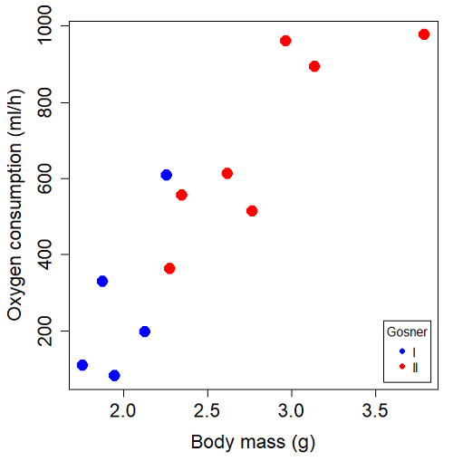
Oxygen consumption of tadpoles by body weight

Figure 1. Scatterplot of oxygen consumption by R. pipiens tadpoles vs body mass (g) by developmental group (Gosner stages I or II).

The project looked at whether metabolism as measured by oxygen consumption was consistent across two developmental stages. Metamorphosis in frogs and other amphibians represents profound reorganization of the organism as the tadpole moves from water to air. Thus, we would predict some cost as evidenced by change in metabolism associated with later stages of development. Figure 2 shows a box plot of tadpole oxygen consumption by Gosner (1960) developmental stage (Figure 2 is a repeat of Figure 4 Chapter 17.5).

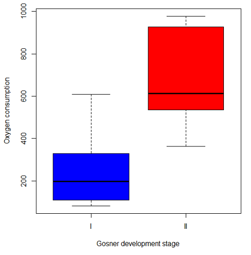
boxplot oxygen consumption of tadploes by developmental stage

Figure 2. Copy of Figure 4, Chapter 17.5; boxplot of oxygen consumption of R. pipiens tadpoles by Gosner developmental stages.

Looking at Figure 2 we see a trend consistent with our prediction; developmental stage may be associated with increased metabolism. However, older tadpoles also tend to be larger, and the plot in Figure 2 does not account for that. Thus, body mass is a confounding variable in this example. There are several options for analysis here (e.g., ANCOVA), but one way to view this is to compare the slopes for the two developmental stages. While this test does not compare the means, it does ask a related question: is there evidence of change in rate of oxygen consumption relative to body size between the two developmental stages? The assumption that the slopes are equal is a necessary step for conducting the ANCOVA.

So, divide the data set (Table 1) into two groups by developmental stage (12 tadpoles could be assigned to one of two developmental stages; one was at a lower Gosner stage than the others and so is dropped from the subset.

Table 1. $\text{Body.mass}$ and $\dot{V} O_{2}$ of 12 R. pipiens tadpole larvae by Gosner developmental stage.

Gosner stage I

$\text{Body.mass}$	$\dot{V} O_{2}$
1.76	109.41
1.88	329.06
1.95	82.35
2.13	198
2.26	607.7

Gosner stage II

Body mass	$\dot{V} O_{2}$
2.28	362.71
2.35	556.6
2.62	612.93
2.77	514.02
2.97	961.01
3.14	892.41
3.79	976.97

The slopes and standard errors we obtained in Chapter 17.5 were

	Gosner Stage I	Gosner stage II
slope	750.0	399.9
standard error of slope	444.6	111.2

Make a plot (Figure 3).

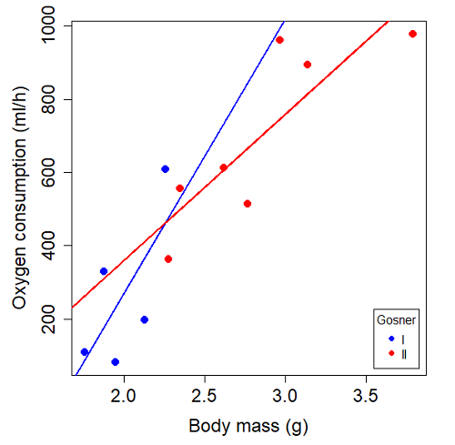
scatterplot oxygen consumption of anuran tadpoles by body mass

Figure 3. Scatterplot with best-fit regression lines of $\dot{V} O_{2}$ by $\text{Body.mass}$ for Gosner State I (closed circle, solid line) and Gosner Stage II (open circle, dashed line) R. pipiens tadpoles.

R code for plot in Figure 3.

#Used Rcmdr scatterplot(), then modified code
scatterplot(VO2~Body.mass | Gosner, regLine=FALSE, smooth=FALSE, 
boxplots=FALSE, xlab="Body mass (g)", ylab="Oxygen consumption (ml/h)", 
main="", cex=1.4, cex.axis=1.5, cex.lab=1.5, pch=c(19,19), by.groups=TRUE,
col=c("blue","red"), grid=FALSE, 
legend=list(coords="bottomright"), data=Tadpoles)
#Get regression equations for groups, subset by Gosner
abline(lm(VO2~Body.mass, data=Stage01), lty=1, lwd=2, col="blue")
abline(lm(VO2~Body.mass, data=Stage02), lty=1, lwd=2, col="red")

Returning to the important question, are the two slopes statistically indistinguishable (Ho: b_I = b_II), where b_I is the slope for the Gosner Stage I subset and b_II is the slope for the Gosner Stage II subset? We look at the plot, and since the lines cross, we tend to see a difference. Of course, we need to consider that our perception of slope differences may simply be chance, especially because the sample size is small. Proceed to test.

R code

The ANCOVA is a new ANOVA model where the factor variables are adjusted or corrected for the effects of the continuous variable.

R code for ANCOVA example, crossed or interaction model.

tadpole.1 <- lm(VO2 ~ Body.mass*Gosner, data=example.Tadpole)
summary(tadpole.1)
Anova(tadpole.1, type="II")

Output

summary(tadpole.1)

Call:
lm(formula = VO2 ~ Body.mass * Gosner, data = example.Tadpole)

Residuals:
    Min      1Q   Median      3Q      Max 
-167.80 -117.93    13.81   94.66   214.65

Coefficients:
                       Estimate   Std. Error   t value    Pr(>|t|) 
(Intercept)             -1231.6       783.0     -1.573    0.1544 
Body.mass                 750.0       390.7      1.919    0.0912 .
Gosner[T.II]              790.4       859.2      0.920    0.3845 
Body.mass:Gosner[T.II]   -350.1       409.5     -0.855    0.4174 
---
Signif. codes: 0 '***' 0.001 '**' 0.01 '*' 0.05 '.' 0.1 ' ' 1

Residual standard error: 155.8 on 8 degrees of freedom
(1 observation deleted due to missingness)
Multiple R-squared: 0.821, Adjusted R-squared: 0.7539 
F-statistic: 12.23 on 3 and 8 DF, p-value: 0.002336

The coefficients for the first factor (GII) and then the differences in the coefficient for the second factor. You can just add the second coefficient to the first so they’re on the same scale.

Anova Table (Type II tests)

Response: VO2
                  Sum Sq   Df    F value     Pr(>F) 
Body.mass         330046    1    13.6030   0.006146 **
Gosner              5630    1     0.2321   0.642908 
Body.mass:Gosner   17736    1     0.7310   0.417423 
Residuals 194102 8 
---
Signif. codes: 0 '***' 0.001 '**' 0.01 '*' 0.05 '.' 0.1 ' ' 1

Suggests interaction is not significant, i.e., the slopes are not different.

We can then proceed to check to see if the intercepts are different, now that we’ve confirmed no significant difference in slope.

R code for ANCOVA as additive model

tadpole.2 <- lm(VO2 ~ Body.mass + Gosner, data=example.Tadpole)
summary(tadpole.2)
Anova(tadpole.2, type="II")

Output

> summary(tadpole.2)

Call:
lm(formula = VO2 ~ Body.mass + Gosner, data = example.Tadpole)

Residuals:
    Min       1Q    Median      3Q      Max 
-163.12  -125.53    -20.27   83.71   228.56

Coefficients:
                   Estimate   Std. Error     t value    Pr(>|t|) 
(Intercept)         -595.37       239.87      -2.482     0.03487 * 
Body.mass            431.20       115.15       3.745     0.00459 **
Gosner[T.II]          64.96       132.83       0.489     0.63648 
---
Signif. codes: 0 '***' 0.001 '**' 0.01 '*' 0.05 '.' 0.1 ' ' 1

Residual standard error: 153.4 on 9 degrees of freedom
(1 observation deleted due to missingness)
Multiple R-squared: 0.8047, Adjusted R-squared: 0.7613 
F-statistic: 18.54 on 2 and 9 DF, p-value: 0.0006432

Anova(tadpole.2, type="II")
Anova Table (Type II tests)

Response: VO2
              Sum Sq    Df    F value      Pr(>F) 
Body.mass     330046     1    14.0221   0.004593 **
Gosner          5630     1     0.2392   0.636482 
Residuals     211839     9 
---
Signif. codes: 0 '***' 0.001 '**' 0.01 '*' 0.05 '.' 0.1 ' ' 1

Note that there is no test of interaction in the added model. This model would be appropriate IF the slopes are equal.

Instead of the interaction, or as added, try as nested model, with body mass nested within stage.

tadpole.3 <- lm(VO2 ~ Body.mass/Gosner, data=example.Tadpole)

summary(tadpole.3)

Call:
lm(formula = VO2 ~ Body.mass/Gosner, data = example.Tadpole)

Residuals:
    Min       1Q    Median      3Q      Max 
-168.66  -131.14    -20.28   90.33   225.36

Coefficients:
                 Estimate      Std. Error    t value Pr(>|t|) 
(Intercept)           -575.10      319.51     -1.800   0.1054 
Body.mass              423.65      162.50      2.607   0.0284 *
Body.mass:Gosner[T.II]  21.95       63.73      0.344   0.7384 
---
Signif. codes: 0 '***' 0.001 '**' 0.01 '*' 0.05 '.' 0.1 ' ' 1

Residual standard error: 154.4 on 9 degrees of freedom
(1 observation deleted due to missingness)
Multiple R-squared: 0.8021, Adjusted R-squared: 0.7581 
F-statistic: 18.24 on 2 and 9 DF, p-value: 0.0006823

Gets the true coefficient (nested lm() version).

The two test different hypotheses.

lm(VO2 ~ Body.mass * Gosner) tests whether or not the regression has a nonzero slope.

lm(VO2 ~ Body.mass */Gosner) test whether or not the slopes and intercepts from different factors are statistically significant.

Questions

An OLS approach was used for the analysis of tadpole oxygen consumption body mass. Consider the RMA approach — would that be a more appropriate regression model? Explain why or why not.
Consider an experiment in which you plan to administer a treatment that has a carry-over effect. For example, Compare and contrast “crossed” and “nested” designs.
True or False. The nested design option for the ANCOVA assumes the slopes for the two groups of tadpoles for the regression line of $\dot{V} O_{2}$ by $\text{Body.mass}$ are equal. Explain your choice.
Metabolic rates like oxygen consumption over time are well-known examples of allometric relationships. That is, many biological variables (e.g., is related as aM^b, where M is body mass, slope b is scaling exponent), and best evaluated on log-log scale. Repeat the analysis above on log₁₀-transformed and for
- crossed design (e.g., tadpole.1 model)
- added design (e.g., tadpole.2 model)
- nested design (e.g., tadpole.3 model)
Create the plot and add the fitted lines from crossed design to the plot.

About log-transform of a variable. The most straight-forward tact is to create two new variables. For example,

lgVO2 <- log(VO2)

Another option is to transform the variables within the call to lm() function. For example, try

lm(log(VO2) ~ log(Body.mass ), data=example.Tadpole)

Hint: don’t forget to attach your data set to avoid having to call the variable as, for example, example.Tadpole$VO2

Data sets

Oxygen consumption, $\dot{V}O_{2}$ , of Anuran tadpoles, dataset=example.Tadpole

Gosner	Body mass	$\{V}O_{2}$
NA	1.46	170.91
I	1.76	109.41
I	1.88	329.06
I	1.95	82.35
I	2.13	198
II	2.28	362.71
I	2.26	607.7
II	2.35	556.6
II	2.62	612.93
II	2.77	514.02
II	2.97	961.01
II	3.14	892.41
II	3.79	976.97

Gosner refers to Gosner (1960), who developed a criteria for judging metamorphosis staging.