9.5 – Fisher exact test

Introduction
R code
When to use the Fisher Exact Test?
Questions
Chapter 9 contents

Introduction

We mentioned that chi-square tests for contingency tables are fine as long as two conditions are met. These are the assumptions of a $\chi^2$ test.

No cell should have expected values less than 5%.
The test performs poorly at DF = 1 because we are approximating an infinite distribution with an exact test.

You will note that any time you have a 2X2 table, the second condition is always an issue because 2X2 tables have DF=1. Thus, in biomedical research, it is common to have an experiment that may be appropriate for a contingency analysis but the data may suffer from one or both of these limitations. Fisher’s exact test is always an option for these types of problems, but with the advantage that it always returns the exact p-value.

A reminder, the 2×2 table looks like

Table 1. 2×2 table reporting numbers of subjects who have (Yes) or do not have (No) the event.

		Column 1	Column 2
	Subjects	Yes	No
Row 1	Treatment 1	a	b
Row 2	Treatment 2	c	d

where a is the count of Treatment 1 – treated subjects who have the event, b is the count of Treatment 1 – treated subjects who do not have the event, c is the count of Treatment 2 – treated subjects who have the event, d is the count of Treatment 2 – treated subjects who do not have the event. Note the row and column totals:

$\begin{align*} Row1 = a + b\\ Row2 = c + d\\ Column1 = a + c\\ Column2 = b + d \end{align*}$

For example, a fairly common, “Gee, that’s curious,” fact is the seven left-handed US Presidents since 1901 (21), is higher than the proportion of left-handers in the general population (about 10%). For comparison, we could ask the same question about Vice Presidents.†

Table 2. U.S. Presidents and Vice-Presidents handedness.

Subjects	Yes	No
Presidents	7	14
Vice presidents	5	20

†Seven Vice-Presidents went on to become President, four right-handers, three left-handers.

Ronald A. Fisher came up with a test that is now called “Fisher’s Exact test” that circumvents this problem. It is an extremely useful test to know about because it provides a way to get an exact probability of the outcome compared to all other possible outcomes. Thus, when asked for a possible alternate to the chi-square contingency test for a 2X2 table, you can respond “Fisher’s Exact test.”

Although tedious to calculate by hand, and resource demanding when done by computer because of the multiple factorial expressions, the major advantage of the test is that it does not rely on the assumption that an underlying distribution applies. The Fisher Exact test can be used to calculate the exact probability of the observed outcome (P).

The equation for the Fisher Exact test can be written as

$\begin{align*} P = \frac{{R_{1}! \cdot R_{2}! \cdot C_{1}! \cdot C_{2}!}}{a! \cdot b \cdot c! \cdot d! \cdot n!} \end{align*}$

where R stands for row total, C stands for column total, n is the sample size, ! is the factorial, and a, b, c, and d are defined as in Table 1.

How does Fisher’s Exact test work? The data are setup in the usual way for a contingency problem, but now, we calculate the probability for all possible outcomes that we COULD have seen from our experiment, and ask if the actual outcome is unusual (low p-value). The trick is recognizing that you have to keep the totals constrained (note row and column totals stay the same).

Table 3. Original 2X2 contingency table (bold), with the next two more extreme outcomes.

original data	$\longrightarrow$	more extreme	$\longrightarrow$	next more extreme still	$\longrightarrow$
Yes	No	Yes	No	Yes	No
10	5	11	4	12	3
4	12	3	13	2	14
	$p-value=0.0206$		$p-value=0.0029$		$p-value=0.0002$

I’ve shown just the one-tailed outcomes, so the p-values are for one-tailed tests of hypothesis. The essence of the test is to find all outcomes MORE extreme than the original, in one direction. The one-tailed P-value then is the sum of all probabilities from those more extreme tables of outcomes.

To get the two-tailed probability, remember that you multiply the one-tailed probability by two. More accurate methods are also available (Agresti 1992).

Calculation of Fisher’s test involves using all possible combinations and factorials. Rcmdr has Fisher’s 2X2 built in via the Contingency table and as part of some Rcmdr plugins (e.g., RcmdrPlugin.EBM, the Evidence Based Medicine plugin). Here we illustrate Fisher Exact test from the context menu in the main Statistics menu.

Alternatively, there are many web sites out there that provide an online calculator for Fisher’s Exact test. Here’s a link to one such calculator on GraphPad’s web site, cookies must be enabled to run this calculator).

To get the Fisher Exact test, your data must already be summarized into a 2X2 table, in which case you can use R Commander via the Contingency tables… menu selection (Fig 1).

Table 4. 2X2 table smokers vs vitamin use.

	Smoker: No	Smoker: Yes
Vitamin use: No	14	26
Vitamin use: Yes	19	15

With the data summarized as in Table 4, we can proceed directly via R Commander to analyze the contingency table, either by Chi-square test of Fisher exact test. First, bring up menu to enter the data (Fig 1):

Rcmdr: Statistics → Contingency tables… → Enter and analyze two-way table…

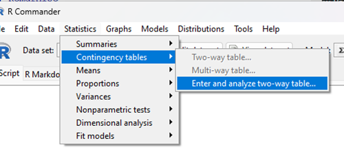
Screenshot Rcmdr Contingency table

Figure 1. Screenshot Rcmdr menu, Contingency tables

The image of the R worksheet below contains two columns: Smoker (No, Yes) and Vitamin use (No, Yes). Complete the form (Fig 2).

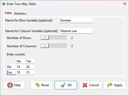
Screenshot Rcmdr menu, Enter two way table

Figure 2. Screenshot Rcmdr menu, Enter Two-Way Table

Alternatively, if the original data are available, do not tally the counts, let R do the work for you. The worksheet would be stacked like so (Table 5).

Table 5. Portion of subject and row entries in stacked worksheet for smokers vs vitamin use.

Subject	Vitamin.use	Smoking
1	No	No
2	No	No
3	No	No
4	No	No
5	No	No
.	.	.
71	Yes	Yes
72	Yes	Yes
73	Yes	Yes
74	Yes	Yes

And from the R Commander menu select as before

Rcmdr: Statistics → Contingency tables… → Two way table …

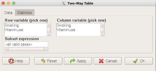
Screenshot Rcmdr two-way table menu, load the data from stacked worksheet.

Figure 3. Screenshot Rcmdr two-way table menu, load the data from stacked worksheet.

Data is now ready.

R code

To carry out contingency table analysis on the entered data (Fig 2 or Fig 3), select the Statistics option tab (Fig 4, green arrow).

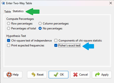
Screenshot Rcmdr menu Statistics option Enter two way table

Figure 4. Screenshot Rcmdr menu Statistics option. Select Chi-square test of independence, Fisher’s exact test, or both.

Check the box next to the Fisher’s exact test (Fig. 4, blue arrow).

Click OK, and here is the R output.

> fisher.test(.Table)
Fisher's Exact Test for Count Data

data: .Table
p-value = 0.1008
alternative hypothesis: true odds ratio is not equal to 1
95 percent confidence interval:
0.1496417 1.1985775
sample estimates:
odds ratio
0.4302094

We accepted the defaults Is this a one or two-tailed test of hypothesis?

What can we conclude about the null hypothesis? Do we accept or reject?

Want to know what the “odds ratio” is? Follow the link to the next subchapter.

When to use the Fisher Exact Test?

Here’s the take-home message: the Fisher exact test is an alternate and better choice over the contingency table chi-square for 2X2 tables if one or more of the cells has expected values less than 5%. It is also appropriate for cases in which you have only 1 degree of freedom (as do all 2X2 tables!), but it doesn’t make sense if each cell has more than 5% expected values (the calculation is too tedious), but rather, apply the Yate’s correction. As the sample sizes get larger, the different methods converge to virtually identical answers.

Some examples.

Is there an association between final grades and attendance on a randomly selected day?

Table 6. First 2X2 scenario.

cc	Yes	No
Letter grade A	2	3
Other letter grade	1	6

Table 7. Second 2X2 scenario.

cc	Yes	No
Letter grade A	5	6
Other letter grade	2	12

Table 8. Third 2X2 scenario.

cc	Yes	No
Letter grade A	10	12
Other letter grade	4	24

Code hints for tests with direct 2X2 entry with matrix() are

grades.Table <- matrix(c(2,3,1,6), 2, 2, byrow=TRUE)

Chi-square test of independence

chisq.test(grades.Table, correct=FALSE)

Fisher Exact test

fisher.test(grades.Table, alternative = "greater")

Questions

1. Apply Fisher exact test on the four contingency tables (a – d) introduced in section 9.3, question 2. Make note of the p-value from Fisher exact test and from analyses used to complete question 2. Note any trends. (Hint: make sure you are testing the same null hypothesis.)

(a)

	Yes	No
A	18	6
B	3	8

(b)

	Yes	No
A	10	12
B	3	14

(c)

	Yes	No
A	5	12
B	12	18

(d)

	Yes	No
A	8	12
B	3	3

9.5 – Fisher exact test

Introduction

R code

When to use the Fisher Exact Test?

Questions

Chapter 9 contents