8.5 – One sample t-test

Introduction

We’re now talking about the traditional, classical two group comparison involving continuous data types. Thus begins your introduction to parametric statistics. One sample tests involve questions like, how many — what proportion of — people would we expect are shorter or taller than two standard deviations from the mean? This type of question assumes a population and we use properties of the normal distribution and, hence, these are called parametric tests because the assumption is that the data has been sampled from a particular probability distribution.

However, when we start asking questions about a sample statistic (e.g., the sample mean), we cannot use the normal distribution directly, i.e., we cannot use Z and the normal table as we did before (Chapter 6.7). This is because we do not know the population standard deviation and therefore must use an estimate of the variation (s) to calculate the standard error of the mean.

With the introduction of the t-statistic, we’re now into full inferential statistics-mode. What we do have are estimates of these parameters. The t-test — aka Student’s t-test — was developed for the purpose of testing sample means when the true population parameters are not known.

The equation of the one sample t-test. Note the resemblance in form with the Z-score!

where  is the sample standard error of the sample mean (SEM).

For example, weight change of mice given a hormone (leptin) or placebo. The  = 5 g, but under the null hypothesis, the mean change is “really” zero ( = 0). How unlikely is our value of 5 g?

Speaking of null hypotheses, can you say (or write) the null and alternative hypotheses in this example? How about in symbolic form?

We want to know if our sample mean could have been obtained by chance alone from a population where the true change in weight was zero.

$s = 3, n = 20$

and

$s_{\overline{X}} = \frac{s}{\sqrt{n}} = \frac{3}{\sqrt{20}} = 0.6708$

and we take these values and plug them into our equation of the t-test

$t = \frac{\left(5 – 0\right)}{0.67} = 7.45$

Then recall that Degrees of Freedom are DF = n – 1 so we have DF = 20 – 1 = 19 for the one sample t-test. And the Critical Value is found in the appropriate table of critical values for the t distribution (Fig. 1)

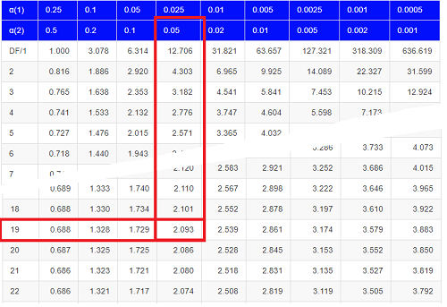
Figure 1. Table of a portion of the Critical values of the t distribution. Red selections highlight critical value for t-test at α = 5% and df = 19.

Or, and better, use R

qt(c(0.025), df=19, lower.tail=FALSE)

where qt() is function call to find t-score of the p^th percentile (cf 3.3 – Measures of dispersion) of the Student t distribution. For a two tailed text, we recall that 0.025 is lower tail and 0.025 is upper tail.

In this example we would be willing to reject the Null Hypothesis if there was a positive OR a negative change in weight.

This was an example of a “two-tailed test” which is “2-tail” or α₍₂₎ in Table of critical values of the t distribution.

Critical Value for α₍₂₎ = 0.05, df = 19, = 2.093

Do we accept or reject the Null Hypothesis?

A typical inference workflow

Note the general form of how the statistical test is processed, a form which actually applies to any statistical inference test.

1. Identify the type of data
2. State the null hypothesis (2 tailed? 1 tailed?)
3. Select the test statistic (t-test) and determine its properties
4. Calculate the test statistic (the value of the result of the t-test)
5. Find degrees of freedom
6. For the DF, get the critical value
7. Compare critical value to test statistic
8. Do we accept or reject the null hypothesis?

And then we ask, given the results of the test of inference, What is the biological interpretation? Statistical significance is not necessarily evidence of biological importance. In addition to statistical significance, the magnitude of the difference — the effect size — is important as part of interpreting results from an experiment. Statistical significance is at least in part because of sample size — the large the sample size, the smaller the standard error of the mean, therefore even small differences may be statistically significant, yet biologically unimportant. Effect size is discussed in Ch9.1 – Chi-square test: Goodness of fit, Ch11.4 – Two sample effect size and Ch12.5 – Effect size for ANOVA.

R Code

Let’s try a one-sample t-test. Consider the following data set: body mass of four geckos and four Anoles lizards (Dohm unpublished data).

For starters, let’s say that you have reason to believe that the true mean for all small lizards is 5 grams (g).

Geckos: 3.186, 2.427, 4.031, 1.995
Anoles: 5.515, 5.659, 6.739, 3.184

Get the data into R (Rcmdr)

By now you should be able to load this data in one of several ways. If you haven’t already entered the data, check out Part 07. Working with your own data in Mike’s Workbook for Biostatistics.

Once we have our data.frame, proceed to carry out the statistical test.

To get the one-sample t-test in Rcmdr, click on Statistics → Means → Single-sample t-test… Because there is only one numerical variable, Body.mass, that is the only one that shows up in the Variable (pick one) window (Fig. 6)

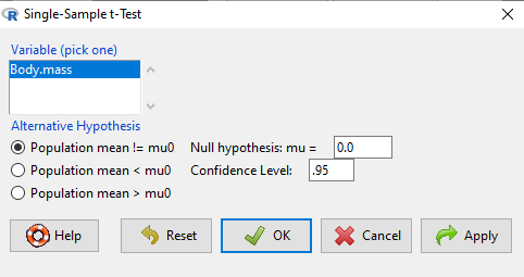
Figure 6. Screenshot Rcmdr single-sample t-test menu

Type in the value 5.0 in the Null hypothesis =mu box.

Question 3: Quick! Can you write, in plain old English, the statistical null hypothesis???

Click OK

The results go to the Output Window.

t.test(lizardsBody.mass
t = -1.5079, df = 7, p-value = 0.1753
alternative hypothesis: true mean is not equal to 5
95 percent confidence interval:
2.668108 5.515892
sample estimates:
mean of x 4.092

end of R output

Let’s identify the parts of the R output from the one sample t-test. R reports the name of the test and identifies

1. The datasetBody.mass). The data set was called “lizards” and the variable was “Body.mass”. R uses the dollar sign (bm, alternative=’two.sided’, mu=5, conf.level=.95)
   And, like the Rcmdr output we have for the one-sample t-test the following R output

   One Sample t-test
   data: lizards$Body.mass
   t = -1.5079, df = 7, p-value = 0.1753 alternative hypothesis: true mean is not equal to 5
   95 percent confidence interval:
   2.668108 5.515892
   sample estimates:
   mean of x
   4.092

   End of R output

   which, as you probably guessed, is the same as what we got from RCmdr.

   Question 9: From the R output of the one sample t-test, what was the value of the test statistic?

   1. -1.5079
   2. 7
   3. 0.1753
   4. 2.668108
   5. 5.515892
   6. 4.092

   Note. On an exam you will be given portions of statistical tables and output from R. Thus you should be able to evaluate statistical inference questions by completing the missing information. For example, if I give you a test statistic value, whether the test is one- or two-tailed, degrees of freedom, and the Type I error rate alpha, you should know that you would need to find the critical value from the appropriate statistical table. On the other hand, if I give you R output, you should know that the p-value and whether it is less than the Type I error rate of alpha would be all that you need to answer the question.

   Think of this as a basic skill.

   In statistics and for some statistical tests, Rcmdr and other software may not provide the information needed to decide that your test statistic is large, and a table in a statistics book is the best way to evaluate the test.

   For now, double check Rcmdr by looking up the critical value from the t-table.

   Check critical value against our test statistic

   Df = 8 – 1 = 7

   The test is two-tailed, therefore α(2)

   α = 0.05 (note that two-tailed critical value is 2.365. T was equal to 1.51 (since t-distribution is symmetrical, we can ignore the negative sign), which is smaller than 2.365 and so we would agree with Rcmdr — we cannot reject the null hypothesis.

   Question 10: From the R output of the one sample t-test, what was the P-value?

   1. -1.5079
   2. 7
   3. 0.1753
   4. 2.668108
   5. 5.515892

   Question 10: We would reject the null hypothesis

   1. False
   2. True

   Questions

   Eleven questions were provided for you within the text in this chapter. Here’s one more.

   12. Here’s a small data set for you to try your hand at the one-sample t-test and Rcmdr. The dataset contains cell counts, five counts of the numbers of beads in a liquid with an automated cell counter (Scepter, Millipore USA). The true value is 200,000 beads per milliliter fluid; the manufacturer claims that the Scepter is accurate within 15%. Does the data conform to the expectations of the manufacturer? Write a hypothesis then test your hypothesis with the one-sample t-test. Here’s the data.

   scepter

   258900

   230300

   107700

   152000

   136400

   ---

   Chapter 8 contents

   • Introduction
   • The null and alternative hypotheses
   • The controversy over proper hypothesis testing
   • Sampling distribution and hypothesis testing
   • Tails of a test
   • One sample t-test
   • Confidence limits for the estimate of population mean
   • References and suggested readings