17.1 – Ordinary least squares regression
-
- Introduction
- Example
- Least squares regression explained
- Models used to predict new values
- R code
- How to extract information from an R object
- Regression equations may be useful to predict new observations
- Regression through the origin
- Assumptions of OLS, an introduction
- Questions
- Quiz
- Chapter 17 contents
Introduction
Linear regression is a toolkit for developing linear models of cause and effect between a ratio scale data type, response or dependent variable, often labeled “Y,” and one or more ratio scale data type, predictor or independent variables, X. Like ANOVA, linear regression is a special case of the general linear model. Regression and correlation both test linear hypotheses: we state that the relationship between two variables is linear (the alternative hypothesis) or it is not (the null hypothesis). The difference?
- Correlation is a test of linear association (are variables correlated, we ask?), but are not tests of causation: we do not imply that one variable causes another to vary, even if the correlation between the two variables is large and positive, for example. Correlations are used in statistics on data sets not collected from explicit experimental designs incorporated to test specific hypotheses of cause and effect.
- Linear regression is to cause and effect as correlation is to association. With regression and ANOVA, which again, are special cases of the general linear model (LM), we are indeed making a case for a particular understanding of the cause of variation in a response variable: modeling cause and effect is the goal.
We start our LM model as 
where “~”, tilda, is an operator used by R in formulas to define the relationship between the response variable and the predictor variable(s).
From R Commander we call the linear model function by Statistics → Fit models → Linear model … , which brings up a menu with several options (Fig 1).
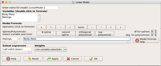
Figure 1. R commander menu interface for linear model.
Our model was
Matings ~ Body.Mass
R commander will keep track of the models created and enter a name for the object. You can, and probably should, change the object name yourself. The example shown in Figure 1 is a simple linear regression, with Body.Mass as the Y variable and Matings the X variable. No other information need be entered and one would simply click OK to begin the analysis.
Example
The purpose of regression is similar to ANOVA. We want a model, a statistical representation to explain the data sample. The model is used to show what causes variation in a response (dependent) variable using one or more predictors (independent variables). In life history theory, mating success is an important trait or characteristic that varies among individuals in a population. For example we may be interested in determining the effect of age (X1) and body size (X2) on mating success for a bird species. We could handle the analysis with ANOVA, but we would lose some information. In a clinical trial, we may predict that increasing Age (X1) and BMI (X2) causes increase blood pressure (Y).
Our causal model looks like

Let’s review the case for ANOVA first.
The response (dependent variable), the number of successful matings for each individual male bird, would be a quantitative (interval scale) variable. (Reminder: You should be able to tell me what kind of analysis you would be doing if the dependent variable was categorical!) If we use ANOVA, then factors have levels. For example, we could have several adult birds differing in age (factor 1) and of different body sizes. Age and body size are quantitative traits, so, in order to use our standard ANOVA, we would have to assign individuals to a few levels. We could group individuals by age (eg, < 6 months, 6 – 10 months, > 12 months) and for body size (eg, small, medium, large). For the second example, we might group the subjects into age classes (20-30, 30-40, etc), and by AMA recommended BMI levels (underweight < 18.5, normal weight 18.5 – 24.9, overweight 25-29.9, obese > 30).
We have not done anything wrong by doing so, but if you are a bit uneasy by this, then your intuition will be rewarded later when we point out that in most cases you are best to leave it as a quantitative trait. We proceed with the test of ANOVA, but we are aware that we’ve lost some information — continuous variables (age, body size, BMI) were converted to categories — and so we suspect (correctly) that we’ve lost some power to reject the null hypothesis. By the way, when you have a “factor” that is a continuous variable, we call it a “covariate.” Factor typically refers to a categorical explanatory (independent) variable.
We might be tempted to use correlation — at least to test if there’s a relationship between Body Mass and Number of Matings. Correlation analysis is used to measure the intensity of association between a pair of variables. Correlation is also used to to test whether the association is greater than that expected by chance alone. We do not express one as causing variation in the other variable, but instead, we ask if the two variables are related (covary). We’ve already talked about some properties of correlation: it ranges from -1 to +1 and the null hypothesis is that the true association between two variables is equal to zero. We will formalize the correlation next time to complete our discussion of the linear relationship between two variables.
But regression is appropriate here because we are indeed making a causal claim: we selected Age and Body Size, and we selected Age and BMI in the second example wish to develop a model so we can predict and maybe even advise.
Least squares regression explained
Regression is part of the general linear model family of tests. If there is one linear predictor variable, then that is a simple linear regression (SLR), also called ordinary least squares (OLS), if there are two or more linear predictor variables, then that is a multiple linear regression (MLR, Chapter 18).
First, consider one predictor variable. We begin by looking at how we might summarize the data by fitting a line to the data; we see that there’s a relationship between mass and mating success in both young and old females (and maybe in older males).
The data set was
Table 1. Our data set of number of matings by male bird by body mass (g).
| Body.Mass | Matings |
|---|---|
| 29 | 0 |
| 29 | 2 |
| 29 | 4 |
| 32 | 4 |
| 32 | 2 |
| 35 | 6 |
| 36 | 3 |
| 38 | 3 |
| 38 | 5 |
| 38 | 8 |
| 40 | 6 |
Note 1: Unfortunately, I’ve lost track where Table 1 data set came from! It’s likely a simulated set inspired by my readings back in 2005.
And a scatterplot of the data (Fig 2)
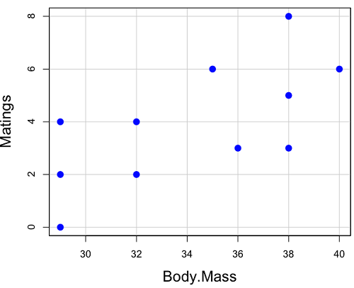
Figure 2. Number of matings by body mass (g) of the male bird.
There’s some scatter, but our eyes tell us that as body size increases, the number of matings also increases. We can go so far as to say that we can predict (imperfectly) that larger birds will have more matings. We fit the best fit line to the data and added the line to our scatterplot (Fig 3). The best fit line meets the requirements that the error about the line is minimized (see below). Thus, we would predict about six matings for a 40 g bird, but only two matings for a 28 g bird. And this is a good feature of regression, prediction, as long as used with some caution.
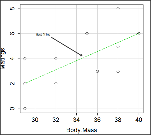
Figure 3. Same data as in Fig 2, but with the “best fit” line.
The prediction works best for the range of data for which the regression model was built. Outside the range of values, we predict with caution.
The simplest linear relationship between two variables is the SLR. This would be the parameter version (population, not samples), where

 = the Y-intercept coefficient and it is defined as

solve for intercept by setting X = 0.
 = the regression coefficient (slope)

Note 2: The denominator is just our corrected sums of squares that we’ve seen many times before. The numerator is the cross-product and is referred to as the covariance.
ε = the error or “residual”

The residual is an important concept in regression. We briefly discussed “what’s left over,” in ANOVA, where an observation Yi is equal to the population mean plus the factor effect of level i plus the remainder or “error”.
In regression, we speak of residuals as the departure (difference) of an actual Yi (observation) from the predicted Y ( , say “why-hat”).
the linear regression predicts Y

and what remains unexplained by the regression equation is called the residual
There will be as many residuals as there were observations.
But why THIS particular line? We could draw lines anywhere through the points. Well, this line is termed the “best fit“ because it is the only line that minimizes the sum of the squared deviations for all values of Y (the observations) and the predicted . The best fit line minimizes the sum of the squared residuals.

Note 3: More technically we justify the OLS as best fit by saying” Following the Gauss–Markov theorem, OLS estimators are the best linear unbiased estimators (BLUE). Gauss (1821) proved that the least squares method produces unbiased estimates with the smallest variance, a key result for regression analysis, while Markov (1900) rediscovered Gauss’ work and showed the conclusions held under less restrictive conditions.
Thus, like ANOVA, we can account for the total sums of squares (SSTot) as equal to the sums of squares (variation), explained by the regression model, SSreg, plus what’s not explained, what’s left over, the residual sums of squares, SSres, aka SSerror.

How well does our model explain — fit — our data? We cover this topic in Chapter 17.3 — Estimation of linear regression coefficients, but for now, we introduce  , the coefficient of determination.

ranges from zero (0%), the linear model fails completely to explain the data, to one (100%), the linear model explains perfectly every datum.
Models used to predict new values
Once a line has been estimated, one use is to predict new observations not previously measured!
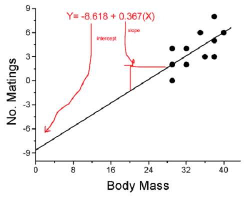
Figure 4. Figure 3 redrawn to extend the line to the Y intercept.
This is an important use of models in statistics: use an equation to fit to some data, then predict Y values from new values of X. To use the equation, simply insert new values of X into the equation, because the slope and intercept are already “known.” Then for any Xi we can determine  (predicted Y value that is on the best fit regression line).
This is what people do when they say
“if you are a certain weight (or BMI) you have this increased risk of heart disease”
“if you have this number of black rats in the forest you will have this many nestlings survive to leave the nest”
“if you have this much run-off pollution into the ocean you have this many corals dying”
“if you add this much enzyme to the solution you will have this much resulting product”.
R Code
We can use the drop down menu in Rcmdr to do the bulk of the work, supplemented with a little R code entered and run from the script window. Scrape data from Table 1 and save to R as bird.matings.
LinearModel.3 <- lm(Matings ~ Body.Mass, data=bird.matings)
summary(LinearModel.3)
Output from R — we’ll pull apart the important parts, color-highlights used to help orient the reader as we go.
Call:
lm(formula = Matings ~ Body.Mass, data = bird.matings)

Residuals:
     Min       1Q   Median      3Q     Max
-2.29237 -1.34322 -0.03178 1.33792 2.70763

Coefficients:
            Estimate Std. Error  t value  Pr(>|t|)
(Intercept)  -8.4746     4.6641   -1.817    0.1026
Body.Mass     0.3623     0.1355    2.673    0.0255 *
---
Signif. codes: 0 '***' 0.001 '**' 0.01 '*' 0.05 '.' 0.1 ' ' 1

Residual standard error: 1.776 on 9 degrees of freedom
Multiple R-squared: 0.4425, Adjusted R-squared: 0.3806
F-statistic: 7.144 on 1 and 9 DF, p-value: 0.02551
What are the values for the coefficients? See Estimate .
Table 2. Coefficient estimates.
| Value | |
 , Y-intercept , Y-intercept |
-8.4746 |
 , Slope , Slope |
0.3623 |
Get the sum of squares from the ANOVA table
myAOV.full <- anova(LinearModel.3); myAOV.full
Output from R, the ANOVA table
Analysis of Variance Table

Response: Matings
           Df  Sum Sq  Mean Sq  F value     Pr(>F)
Body.Mass   1  22.528  22.5277   7.1438   0.02551 *
Residuals   9  28.381   3.1535
---
Signif. codes: 0 '***' 0.001 '**' 0.01 '*' 0.05 '.' 0.1 ' ' 1
Looking for , the coefficient of determination? From the R output identify Multiple R-squared. We find 0.4425. Grab the SSreg and SSTot from the ANOVA table and confirm

Note 2: The value of increases with each additional predictor variable included in the model, whether statistically significant contributor or not, regardless of whether the association between the predictor is simply due to chance. The Adjusted R-squared is an attempt to correct for this bias.
The residual standard error, RSE, is another model fit statistic.

The smaller the residual standard error, the better the model fit to the data. See Residual standard error: 1.776 and MSE = 3.1535 above.
And the “statistical significance?” See Pr(>|t|) .There were tests for each coefficient,  and
and  :
:
Table 3. Coefficient estimates.
| P-value | |
| , Y-intercept |
0.1026 |
| , Slope |
0.0255 |
And, at last, note that p-value, Pr(>F), reported in the Analysis of Variance Table, is the same as the p-value for the slope reported as Pr(>|t|).
Make a prediction:
How many matings expected for a 40 g male?
predict(LinearModel.3, data.frame(Body.Mass=40))
R output
1
6.016949
Answer: we predict 6 matings for a 40g male.
See below for predicting confidence limits.
How to extract information from an R object
We can do more — the lm() returnd a great deal of information about our regression model. Explore all that is available in the objects LinearModel.3 and myAOV.full with the str() command.
Note 3: str() command lets us look at an object created in R. Type ?str or help(str) to bring up the R documentation. Here, we use str() to look at the structure of the objects we created. “Classes” refers to the R programming class attribute inherited by the object. We first used str() in Chapter 8.3.
str(LinearModel.3)
Output from R
List of 12
$ coefficients : Named num [1:2] -8.475 0.362
..- attr(*, "names")= chr [1:2] "(Intercept)" "Body.Mass"
$ residuals : Named num [1:11] -2.0318 -0.0318 1.9682 0.8814 -1.1186 ...
..- attr(*, "names")= chr [1:11] "1" "2" "3" "4" ...
$ effects : Named num [1:11] -12.965 4.746 2.337 1.327 -0.673 ...
..- attr(*, "names")= chr [1:11] "(Intercept)" "Body.Mass" "" "" ...
$ rank : int 2
$ fitted.values: Named num [1:11] 2.03 2.03 2.03 3.12 3.12 ...
..- attr(*, "names")= chr [1:11] "1" "2" "3" "4" ...
$ assign : int [1:2] 0 1
$ qr :List of 5
..$ qr : num [1:11, 1:2] -3.317 0.302 0.302 0.302 0.302 ...
.. ..- attr(*, "dimnames")=List of 2
.. .. ..$ : chr [1:11] "1" "2" "3" "4" ...
.. .. ..$ : chr [1:2] "(Intercept)" "Body.Mass"
.. ..- attr(*, "assign")= int [1:2] 0 1
..$ qraux: num [1:2] 1.3 1.3
..$ pivot: int [1:2] 1 2
..$ tol : num 0.0000001
..$ rank : int 2
..- attr(*, "class")= chr "qr"
$ df.residual : int 9
$ xlevels : Named list()
$ call : language lm(formula = Matings ~ Body.Mass, data = bird_matings)
$ terms :Classes 'terms', 'formula' language Matings ~ Body.Mass
.. ..- attr(*, "variables")= language list(Matings, Body.Mass)
.. ..- attr(*, "factors")= int [1:2, 1] 0 1
.. .. ..- attr(*, "dimnames")=List of 2
.. .. .. ..$ : chr [1:2] "Matings" "Body.Mass"
.. .. .. ..$ : chr "Body.Mass"
.. ..- attr(*, "term.labels")= chr "Body.Mass"
.. ..- attr(*, "order")= int 1
.. ..- attr(*, "intercept")= int 1
.. ..- attr(*, "response")= int 1
.. ..- attr(*, ".Environment")=<environment: R_GlobalEnv>
.. ..- attr(*, "predvars")= language list(Matings, Body.Mass)
.. ..- attr(*, "dataClasses")= Named chr [1:2] "numeric" "numeric"
.. .. ..- attr(*, "names")= chr [1:2] "Matings" "Body.Mass"
$ model :'data.frame': 11 obs. of 2 variables:
..$ Matings : num [1:11] 0 2 4 4 2 6 3 3 5 8 ...
..$ Body.Mass: num [1:11] 29 29 29 32 32 35 36 38 38 38 ...
..- attr(*, "terms")=Classes 'terms', 'formula' language Matings ~ Body.Mass
.. .. ..- attr(*, "variables")= language list(Matings, Body.Mass)
.. .. ..- attr(*, "factors")= int [1:2, 1] 0 1
.. .. .. ..- attr(*, "dimnames")=List of 2
.. .. .. .. ..$ : chr [1:2] "Matings" "Body.Mass"
.. .. .. .. ..$ : chr "Body.Mass"
.. .. ..- attr(*, "term.labels")= chr "Body.Mass"
.. .. ..- attr(*, "order")= int 1
.. .. ..- attr(*, "intercept")= int 1
.. .. ..- attr(*, "response")= int 1
.. .. ..- attr(*, ".Environment")=<environment: R_GlobalEnv>
.. .. ..- attr(*, "predvars")= language list(Matings, Body.Mass)
.. .. ..- attr(*, "dataClasses")= Named chr [1:2] "numeric" "numeric"
.. .. .. ..- attr(*, "names")= chr [1:2] "Matings" "Body.Mass"
- attr(*, "class")= chr "lm"
Yikes! A lot of the output is simply identifying how R handled our data.frame and applied the lm() function.
Note 4: The “how” refers to the particular algorithms used by R. For example, qraux, pivot, and tol refer to arguments used in the QR decomposition of the matrix (derived from our data.frame) used to solve our linear least squares problem.
However, it’s from this command we learn what is available to extract in our object. For example, what were the actual fitted values (, the predicted Y values) from our linear equation? I marked the relevant str() output above in yellow. We call these from the object with the R code
RegModel.1$fitted.values
and R returns
       1        2        3        4        5        6        7        8        9       10       11
2.031780 2.031780 2.031780 3.118644 3.118644 4.205508 4.567797 5.292373 5.292373 5.292373 6.016949
Here’s another look at an object, str(myAOV.full), and how to extract useful values.
Output from R
Classes 'anova' and 'data.frame': 2 obs. of 5 variables:
$ Df : int 1 9
$ Sum Sq : num 22.5 28.4
$ Mean Sq: num 22.53 3.15
$ F value: num 7.14 NA
$ Pr(>F) : num 0.0255 NA
- attr(*, "heading")= chr [1:2] "Analysis of Variance Table\n" "Response: Matings"
Extract the sum of squares: type the object name then $ Sum Sq at the R prompt.
myAOV.full $"Sum Sq"
Output from R
[1] 22.52773 28.38136
Get the residual sum of squares
SSE.myAOV.full <- myAOV.full $"Sum Sq"[2]; SSE.myAOV.full
Output from R
[1] 22.52773
Get the regression sum of squares
SSR.myAOV.full <- myAOV.full $"Sum Sq"[1]; SSR.myAOV.full
Output from R
[1] 50.90909
Now, get the total sums of squares for the model

ssTotal.myAOV.full <- SSE.myAOV.full + SSR.myAOV.full; ssTotal.myAOV.full
Calculate the coefficient of determination
myR_2 <- 1 - (SSE.myAOV.full/(ssTotal.myAOV.full)); myR_2
Output from R
[1] 0.4425091
Which matches what we got before, as it should.
Regression equations may be useful to predict new observations
True. However, you should avoid making estimates beyond the range of the X – values that were used to calculate the best fit regression equation! Why? The answer has to do with the shape of the confidence interval around the regression line.
I’ve drawn an exaggerated confidence interval (CI), for a regression line between an X and a Y variable. Note that the CI is narrow in the middle, but wider at the end. Thus, we have more confidence in predicting new Y values for data that fall within the original data because this is the region where we are most confident.
Calculating the CI for the linear model follows from CI calculations for other estimates. It is a simple concept — both the intercept and slope were estimated with error, so we combine these into a way to generalize our confidence in the regression model as a whole given the error in slope and intercept estimation.

The calculation of confidence interval for the linear regression involves the standard error of the residuals, the sample size, and expressions relating the standard deviation of the predictor variable X — we use the t distribution.
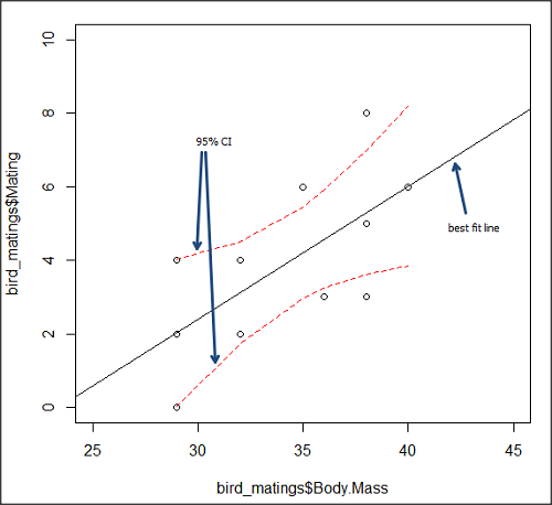
Figure 5. 95% confidence interval about the best fit line.
How I got this graph
plot(bird_matings$Body.Mass,bird_matings$Mating,xlim=c(25,45),ylim=c(0,10))
mylm <- lm(bird_matings$Mating~bird_matings$Body.Mass)
predict(mylm, interval = c("confidence"))
abline(mylm, col = "black")
x<-bird_matings$Body.Mass
lines(x, prd[,2], col= "red", lty=2)
lines(x, prd[,3], col= "red", lty=2)
Nothing wrong with my code, but getting all of this to work in R might best be accomplished by adding another package, a plug-in for Rcmdr called RcmdrPlugin.HH. HH refers to “Heiberger and Holland,” and provides software support for their textbook Statistical Analysis and Data Display, 2nd edition.
Regression through the origin
A regression through the origin in OLS is appropriate when theory dictates that the response must be zero when the predictor is zero, that is, the intercept is known to be exactly 0. In population genetics, for example, if you model pairwise genetic distance as a function of some measure of separation, (eg, time or geographic distance), and the definition of the metric ensures that identical individuals have zero distance, then forcing the regression through the origin can be justified. Doing so reduces parameter estimation to the slope alone and can improve efficiency when the assumption is correct. However, if the true relationship includes a nonzero intercept, constraining it to zero biases the slope.
This choice also affects the coefficient of determination (R²): in a no-intercept model, R² is computed relative to zero rather than the mean of Y, so it is not directly comparable to the standard R² from a model with an intercept and can even appear artificially higher or lower. If the origin constraint is correct, the no-intercept model may show a better (more meaningful) fit; if not, the apparent R² can be misleading despite biased estimates.
R code for regression without the Y-intercept:
noOrigin.model <- lm(formula = Matings ~ 0 + Body.Mass, data = bird.matings)
summary(noOrigin.model)
And the R output:
Call:
lm(formula = Matings ~ 0 + Body.Mass, data = bird.matings)

Residuals:
    Min      1Q  Median      3Q     Max
-3.4112 -1.4406  0.2359  0.9418  3.5301

Coefficients:
          Estimate Std. Error t value Pr(>|t|)
Body.Mass  0.11763    0.01726   6.816 4.65e-05 ***
---
Signif. codes:  0 ‘***’ 0.001 ‘**’ 0.01 ‘*’ 0.05 ‘.’ 0.1 ‘ ’ 1

Residual standard error: 1.97 on 10 degrees of freedom
Multiple R-squared:  0.8229,	Adjusted R-squared:  0.8052
F-statistic: 46.45 on 1 and 10 DF,  p-value: 4.65e-05
Interpretation and comparison between model with and without fit through the origin.
Without an intercept (regression through the origin), the model estimates a slope of 0.1176 (SE = 0.0173, t = 6.82, p = 4.65×10⁻⁵), indicating a strong, statistically significant positive association between Body Mass and the response. Because the intercept is constrained to zero, this slope is effectively forced to account for all variation in Y, which often inflates its magnitude of significance and can bias the estimate if the true relationship does not pass through the origin.
When the intercept was included, the slope increased to 0.3623 (SE = 0.1355, t = 2.67, p = 0.0255), still statistically significant but less so, while the intercept is estimated at –8.47 (SE = 4.66, p = 0.103), which is not significantly different from zero at conventional levels. The change in slope (from 0.12 to 0.36) shows that allowing a nonzero intercept alters the fitted relationship substantially, suggesting that the origin constraint may not be appropriate in this case. Even though the intercept is not statistically significant, its inclusion redistributes variance between intercept and slope, yielding a more reliable slope estimate and a standard R² that is comparable across models, unlike the no-intercept case.
The negative Y-intercept, while statistically justifiable, is also biologically unrealistic, implying a negative number of matings. The statistical justification is simply that the model is used to predict mating success for organisms in the range of body size included in the data set used to make the model — the negative Y-intercept than is interpreted that we are trying to extend the model beyond its range.
In our example with the birds, a biological justification for a non intercept model can be made. For example, mating success is positively associated with body size; therefore, an organism with a hypothetical body size of zero would logically have zero chance of mating success. That said, even when biology suggests the relationship should pass through the origin, it may still be useful to fit a model with an intercept to test that assumption rather than impose it.
Measurement error, in the case of our birds example, chiefly if observed count of matings differs from the true, actual number of matings that occurred, or in a student employing genetic distance, then a number of errors may occur, including sequencing artifacts, alignment bias, or the way genetic distance is computed (eg, corrections for multiple substitutions, cf discussions in Felsenstein 2003, see Legendre and Desdevises 2009 for justifications for through the origin and phylogenetic independent contrasts). As well documented in standard texts on regression and linear models (eg, Introduction to Linear Regression Analysis, by Montgomery et al 2021; An Introduction to Generalized Linear Models, by Dobson and Barnett 2018), measurement error can introduce a small offset, so the estimated intercept serves as a diagnostic for systematic bias. If the intercept is close to zero and not significant, that provides empirical support for the origin constraint; if it is meaningfully different from zero, forcing the regression through the origin would bias the slope and distort inference. Additionally, including the intercept yields a standard R² and residual structure that are comparable across models, helping assess overall model fit before deciding whether the biologically motivated constraint is justified.
Assumptions of OLS, an introduction
We will cover assumptions of Ordinary Least Squares in detail in 17.8, Assumptions and model diagnostics for Simple Linear Regression. For now, briefly, the assumptions for OLS regression include:
- Linear model is appropriate: the data are well described (fit) by a linear model
- Independent values of Y and equal variances. Although there can be more than one Y for any value of X, the Y’s cannot be related to each other (that’s what we mean by independent). Since we allow for multiple Y’s for each X, then we assume that the variances of the range of Ys are equal for each X value (this is similar to our ANOVA assumptions for equal variance by groups).
- Normality. For each X value there is a normal distribution of Ys (think of doing the experiment over and over)
- Error (residuals) are normally distributed with a mean of zero.
Additionally, we assume that measurement of X is done without error (the equivalent, but less restrictive practical application of this assumption is that the error in X is at least negligible compared to the measurements in the dependent variable). Multiple regression makes one more assumption, about the relationship between the predictor variables (the X variables). The assumption is that there is no multicolinearity: the X variables are not related or associated to each other.
In some sense the first assumption is obvious if not trivial — of course a “line” needs to fit the data so why not plow ahead with the OLS regression method, which has desirable statistical properties and let the estimation of slopes, intercept and fit statistics guide us? One of the really good things about statistics is that you can readily test your intuition about a particular method using data simulated to meet, or not to meet, assumptions.
What about assumptions and BLUE? Interestingly, OLS coefficient estimates remain unbiased even if the errors are not normal, as long as other assumptions (like a mean of zero, no correlation, and constant variance) hold. However, the OLS estimators are no longer the “best” linear unbiased estimators (BLUE) because the efficiency property is lost. As we have discussed before, the main consequence is the effects on statistical inference. Without normality, standard errors, t-statistics, confidence intervals, and p-values will be unreliable.
Note 5: The efficiency property means the estimator has the smallest variance among all linear, unbiased estimators. And “unbiased,” again, means the estimator’s expected value is equal to the true parameter value.
Coming up with datasets like these can be tricky for beginners. Thankfully, others have stepped in and provide tools useful for data simulations which greatly facilitate the kinds of testing of assumptions — and more importantly, how assumptions influence our conclusions — statisticians greatly encourage us all to do (see Chatterjee and Firat 2007).
Questions
- Write up three learning outcomes for this page. Hint: Point your favorite generative AI to this page and ask for help.
- Predict new values for number of matings for male birds of 20g and 60g.
- Anscombe’s quartet (Anscombe 1973) is a famous example of this approach and the fictitious data can be used to illustrate the fallacy of relying solely on fit statistics and coefficient estimates.
Here are the data (modified from Anscombe 1973, p. 19) — I leave it to you to discover the message by using linear regression on Anscombe’s data set. Hint: play naïve and generate the appropriate descriptive statistics, make scatterplots for each X, Y set, then run regression statistics, first on each of the X, Y pairs (there were four sets of X, Y pairs).
Anscombe’s quartet
| X | Y1 | Y2 | Y3 | Y4 |
|---|---|---|---|---|
| 10 | 8.04 | 9.14 | 7.46 | 6.58 |
| 8 | 6.95 | 8.14 | 6.77 | 5.76 |
| 13 | 7.58 | 8.74 | 12.74 | 7.71 |
| 9 | 8.81 | 8.77 | 7.11 | 8.84 |
| 11 | 8.33 | 9.26 | 7.81 | 8.47 |
| 14 | 9.96 | 8.10 | 8.84 | 7.04 |
| 6 | 7.24 | 6.13 | 6.08 | 5.25 |
| 4 | 4.26 | 3.10 | 5.39 | 12.50 |
| 12 | 10.84 | 9.13 | 8.15 | 5.56 |
| 7 | 4.82 | 7.26 | 6.42 | 7.91 |
| 5 | 5.68 | 4.74 | 5.73 | 6.89 |
| Mean (±SD) | 7.50 (2.032) | 7.50 (2.032) | 7.50 (2.032) | 7.50 (2.032) |
Quiz Chapter 17.1
Ordinary Least Squares
Chapter 17 contents
- Introduction
- Simple Linear Regression
- Relationship between the slope and the correlation
- Estimation of linear regression coefficients
- OLS, RMA, and smoothing functions
- Testing regression coefficients
- ANCOVA – analysis of covariance
- Regression model fit
- Assumptions and model diagnostics for Simple Linear Regression
- References and suggested readings (Ch17 & 18)