6.7 – Normal distribution and the normal deviate (Z)
Introduction
In chapter 3.3 we introduced the normal distribution and the Z score, aka normal deviate, as part of a discussion about how some knowledge about characteristics of the dispersion of our data sampled from a population could be used to calculate how many samples we need (the empirical rule). We introduced Chebyshev’s inequality as a general approach to this problem, where little is known about the distribution of the population and contrasted it with the Z score, for cases where the distribution is known to be Gaussian or the normal distribution. The normal distribution is one of the most important distributions in classical statistics. All normal distributions are bell-shaped and symmetric about the mean. To describe a normal distribution only two parameters are needed: the population mean, μ, and the population standard deviation, σ. The normal distribution with mean equal to zero and standard deviation equal to one is called the standard normal, or Z distribution. With use of the Z score any normal distribution can be quickly converted to the standard normal distribution.
Proportions of a Normal Distribution
This concept will become increasingly important for the many statistical tests we will learn over the next few weeks. What is the proportion of the populations that is greater than some specific value? Below (Fig 1), again, I have generated a large data set, now with population mean µ = 5 and σ = 2. The red line corresponds to the equation of the normal curve using our values of µ = 5 and σ = 2.

Figure 1. Frequency of observations expected to be greater than 7 (red bars) from a large population with mean µ = 5 and σ = 2.
R code for Fig 1.
set.seed(123)
myData <- rnorm(1000, mean = 5, sd = 2)
h <- hist(myData, breaks = 20, plot = FALSE)
threshold <- 7
# Bars with midpoints greater than threshold will be "red",
# and others will be "white."
bar_colors <- ifelse(h$mids > threshold, "red", "white")
plot(h, col = bar_colors, xlab = "Value", ylab = "Frequency")
Note that this is a crucial step! We assume that our sample distribution is really a sample from a population density (= “area under the curve”) function (= “an equation”) for a normal random (= “population”) variable.
Once I (you) make this assumption, then we have powerful and easy to use tools at our command to answer questions like
Question: What proportion of the population is greater than 7 (Fig 1, colored in red)?
This gets to the heart of the often-asked question, How many samples should I measure? If we know something about the mean and the variability, then we can predict how many samples will be of a particular kind. Let’s solve the problem.
The Z score
We could use the formula for the normal curve (and a lot of repetitions), but fortunately, some folks have provided tables that short-cut this procedure. R and other programs also can find these numbers because the formulas are “built in” to the base packages. First, let’s introduce a simple formula that lets us standardize our population numbers so that we can use established tables of probabilities for the normal distribution.
Below, we will see how to use Rcmdr for these kinds of problems.
However, it’s one of the basic tasks in statistics that you should be able to do by hand. We’ll use the Z score as a way to take advantage of known properties of the standard normal curve.

Z = 1 (with the mean and SD). Z (say “Z-score”) is called the normal deviate (aka “standard normal score”; it is also called the “Z-score”); it gives us a shortcut for finding the proportion of data greater than 7 in this case).
We use the normal deviate to do a couple of things; one use is to standardize a sample of observations so that they have a mean of zero and a standard deviation of one (the Z distribution). The data would then said to have been normalized.
The second use is to make predictions about how often a particular observation is likely to be encountered. As you can imagine, this last use is very helpful for designing an experiment — if we need to see a specified difference, we can conduct a pilot study (or refer to the literature) to determine a mean and level of variability for our observation of choice, plug these back into the normal equation and predict how likely we can expect to see a particular difference. In other words, this is one way to answer that question — how many observations need I make for my experiment to be valid?
Table of normal distribution
A portion of the table of the normal curve is provided at our web site and in your workbook. For our discussions, here’s another copy to look at (Fig 2).
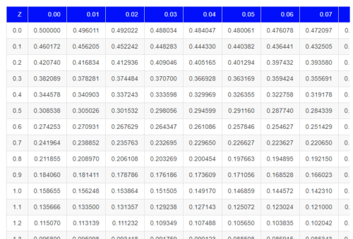
Figure 2. Portion of the table of the normal distribution. Only values equal to or greater than Z = 0 are visible.
See Table 1 in the Appendix for a full version of the normal table.
We read values of Z from the first column and the first row. For Z = 0.23 we would scan the top row, scoot over to fourth column, then trace to where the row and column intersect (Fig 3); the frequency of occurrence of values at Z = 0.23 is 0.409046 or 40.9% (Fig 3).
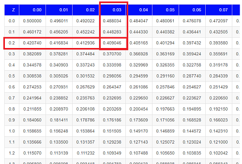
Figure 3. Highlight Z = 0.23, frequency is 0.409046.
Z on the standard normal table is going to range between -4 and +4, with Z = 0 corresponding to 0.500. The Normal table values are symmetrical about the mean of zero.
What to make of the values of Z, from -4, -3, … +2, +3, up to +4 and beyond? These are the standard deviations! Recall that using the Z score you corrected to mean of zero (got it!), and a standard deviation of one! A Z of 2 is twice the standard deviation; a Z = 3 is therefore three times the standard deviation, and so forth. The distribution is symmetrical: you get the same frequency for negative as for positive values. So on the “X” axis on a standard normal distribution, we have units of standard deviation plus (greater) or minus (less) than the mean. In Figure 4, area less than -1 standard deviations is highlighted (Fig 4).
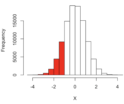
Figure 4. Plot of standard normal distribution; area less than -1 σ.
R code for Fig 4.
set.seed(123)
myData2 <- rnorm(100000, mean = 0, sd = 1)
threshold <- -1
bar_colors <- ifelse(h$mids < threshold, "red", "white")
# Additional code used, same as Figure 1.
Question. How many multiples of standard deviations would you have for a Z score of Z = 1.75?
Answer = 1.75 times
Examples
See Table 1 in the Appendix for a full version of the normal table as you read this section.
What proportion of the data set will have values greater than 7? After applying our Z score equation, I get Z = 1.0 and for a Z of 1.0 = 0.1587 or 15.87% of the observations are greater than 7.
What proportion of the data set will have values less than -7? After applying our Z score equation, I get Z = -1.0. Taking advantage of symmetry argument, I just take my Z = -1.0 and make it positive — instead of values smaller than -1.0 we now have values greater than +1.0. And for a Z of 1.0 = 0.1587 or 15.87% of the observations are greater than 7, which means that 15.87% will be -7 or smaller.
What proportion of the data set will have values greater than 8? Again, apply the Z score equation I get Z of 1.5 = 0.0668 or 6.68% of the observations are greater than Z.
What proportion of the population is between 5 and 7 ? (colored in red). Draw the problem (example shown in Fig 5).
Figure 5. Proportion of the population is between 5 and 7.
R code for Fig 5.
# Used myData from Fig 1 code.
highlight_start <- 5
highlight_end <- 7
bar_colors <- rep("white", length(h$counts))
bar_colors[h$breaks[-length(h$breaks)] >= highlight_start & h$breaks[-1] <= highlight_end] <- "red"
# Additional code used, same as Figure 1.
Note 1: h$breaks[-length(h$breaks)] gives the left edges of the bins, and h$breaks[-1] gives the right edges.
Worked problem
1 – (proportion beyond 7) – (proportion less than 5)
1 – (0.1587) – (proportion less than 5)
And the proportion less than 5?
Use Z-score equation again. Now we find that
Z = 0
And look up Z of 0 from the table = 0.5 proportion or 50.0%
Therefore, the proportion between 5 & 7 equals
1 -0.1587 – 0.50 = 0.3413
Answer = 34.13 % of the observations are between 5 and 7 when the mean µ = 5 and s = 2.
Questions
Several questions were asked in the text.
1. Proportion of observations greater than 7 from a large population with mean µ = 5 and σ = 2.
2. How many multiples of standard deviations would you have for a Z score of Z = 1.75?
3.
Quiz Chapter 6.7
Normal distribution questions
Chapter 6 contents
- Introduction
- Some preliminaries
- Ratios and probabilities
- Combinations and permutations
- Types of probability
- Discrete probability distributions
- Continuous distributions
- Normal distribution and the normal deviate (Z)
- Moments
- Chi-square (Χ2) distribution
- t distribution
- F distribution
- References and suggested readings