17.4 – OLS, RMA, and smoothing functions

Introduction
Generalized Least Squares
Weighted Least Squares
Reduced Major Axis
Smoothing functions
Questions
Data set
Chapter 17 contents

Introduction

OLS or ordinary least squares is the most commonly used estimation procedure for fitting a line to the data. For both simple and multiple regression, OLS works by minimizing the sum of the squared residuals. OLS is appropriate when the linear regression assumptions LINE apply. In addition, further restrictions apply to OLS including that the predictor variables are fixed and without error. OLS is appropriate when the goal of the analysis is to retrieve a predictive model. OLS describes an asymmetric association between the predictor and the response variable: the slope b_X for Y ~ b_XX will generally not be the same as the slope b_Y for X ~ b_YY.

OLS is appropriate for assessing functional relationships (i.e., inference about the coefficients) as long as the assumptions hold. In some literature, OLS is referred to as a Model I regression.

Generalized Least Squares

Generalized linear regression is an estimation procedure related to OLS but can be used either when variances are unequal or multicollinearity is present among the error terms.

Weighted Least Squares

A conceptually straightforward extension of OLS can be made to account for situation where the variances in the error terms are not equal. If the variance of Yi varies for each Xi, then a weighting function based on the reciprocal of the estimated variance may be used.

$\begin{align*} w_{i} = \frac{1}{s_{i}^2} \end{align*}$

then, instead of minimizing the squared residuals as in OLS, the regression equation estimates in weighted least squares minimizes the squared residuals summed over the weights.

$\begin{align*} \sum w_{i} \left (y_{i} - \hat{y}_{i} \right )^2 \end{align*}$

Weighted least squares is a form of generalized least squares. In order to estimate w_i, however, multiple values of Y for each observed X must be available.

Reduced Major Axis

There are many alternative methods available when OLS may not be justified. These approaches, collectively, may be called Model II regression methods. These methods are invariably invoked in situations in which both Y and X variables have random error associated with them. In other words, the OLS assumption that the predictor variables are measured without error is violated. Among the more common methods is one called Reduced Major Axis or RMA.

Smoothing functions

data set: atmospheric carbon dioxide (CO₂) readings Mauna Loa. Source: http://co2now.org/Current-CO2/CO2-Now/noaa-mauna-loa-co2-data.html

Fit curves without applying a known formula. This technique is called smoothing and, while there are several versions, the technique involves taking information from groups of observations and using these groups to estimate how the response variable changes with values of the independent variable. Techniques by name include kernel, loess, and spline. Default in the scatter plot command is loess.

CO₂ in parts per million (ppm) plotted by year from 1958 to 2014 the first CO₂ readings were recorded in April 1958; the last data available for this plot was April 2014) (Fig. 1).

Note: CO₂ 416.71 ppm December 2021, a 0.6% since December 2020; https://www.esrl.noaa.gov/gmd/ccgg/trends/

A few words of explanation for Figure 1. The green line shows the OLS line, the red line shows the loess smoothing with a smoothing parameter of 0.5 (in Rcmdr the slider value reads “5”).

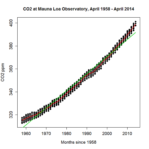
CO2 in parts per million (ppm) plotted by year from 1958 to 2014

Figure 1. CO₂ in parts per million (ppm) plotted by year from 1958 to 2014

R command was started with option settings available in Rcmdr context menu for scatterplot, then additional commands were added

scatterplot(CO2~Year, reg.line=lm, grid=FALSE, smooth=TRUE, spread=FALSE, boxplots=FALSE, span=0.05, lwd=2, xlab="Months since 1958", ylab="CO2 ppm", main="CO2 at Mauna Loa Observatory, April 1958 - April 2014", cex=1, cex.axis=1.2, cex.lab=1.2, pch=c(16), data=StkCO2MLO)

The next plot is for ppm CO₂ by month for the year 2013. The plot shows the annual cycle of atmospheric CO₂ in the northern hemisphere.

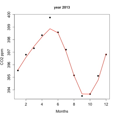
Plot of ppm CO2 by month for the year 2013

Figure 2. Plot of ppm CO₂ by month for the year 2013.

Again, the smoothing parameter was set to 0.5 and the loess function is plotted in red (Fig. 2).

Loess is an acronym short for local regression. Loess is a weighted least squares approach which is used to fit linear or quadratic functions of the predictors at the centers of neighborhoods. The radius of each neighborhood is chosen so that the neighborhood contains a specified percentage of the data points. This percentage of data points is referred to as the smoothing parameter and this parameter may differ for different neighborhoods of points. The idea of loess, in fact, any smoothing algorithm, is to reveal pattern within a noisy sequence of observations. The smoothing parameter can be set to different values, between 0 and 1 is typical.

Note: Noisy data in this context refers to data comes with random error independent of the true signal, i.e., noisy data has low signal-to-noise ratio. The concept is most familiar in communication.

To get a sense of what the parameter does, Figure 3 takes the same data as in Figure 2, but with different values of the smoothing parameter (Fig. 3).

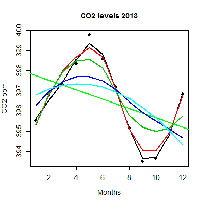
Timeseries plot ppm carbon dioxide by month for year 2013 with different smoothing values (0.5 to 10.0).

key:

parameter	color
0.5	black
0.75	red
1.0	dark green
2.0	blue
10.0	light blue

Figure 3. Plot with different smoothing values (0.5 to 10.0).

The R code used to generate Figure 3 plot was

spanList = c(0.5, 0.75, 1, 2, 10)
reg1 = lm(ppm~Month)
png(filename = "RplotCO2mo.png", width = 400, height = 400, units = "px", pointsize = 12, bg = "white")
plot(Month,ppm, cex=1.2, cex.axis=1.2, cex.lab=1.2, pch=c(16), xlab="Months", ylab="CO2 ppm", main="CO2 levels 2013")
abline(reg1,lwd=2,col="green") 
for (i in 1:length(spanList))
{
ppm.loess <- loess(ppm~Month, span=spanList[i], Dataset)  
ppm.predict <- predict(ppm.loess, Month)
lines(Month,ppm.predict,lwd=2,col=i)
}

Note: This is our first introduction to use of a “for” loop.

The CO2 data constitutes a time series. Instead of loess, a simple moving average would be a more natural way to reveal trends. In principle, take a set of nearby points (odd number of points best, keeps the calculation symmetric) and calculate the average. Next, shift the points by a specified time interval (e.g., 7 days), and recalculate the average for the new set of points. See Chapter 20.5 for Time series analysis.

Questions

This is a biology class, so I gotta ask: What environmental process explains the shape of the relationship between ppm CO₂ and months of the year as shown in Figure 2? Hint: NOAA Global Monitoring Laboratory responsible for the CO2 data is located at Mauna Loa Observatory, Hawaii (lat: 19.52291, lon: -155.61586).
As I write this question (January 2022), we are 22 months since W.H.O. declared Covid-19 a pandemic (CDC timeline). Omicron variant is now dominant; Daily case counts State of Hawaii from 1 November 2021 to 15 January 2022 reported in data set table.
1. Make plot like Figure 2 (days instead of months)
2. Apply different loess smoothing parameters and re-plot the data. Observe and describe the change to the trend between case reports and days.

Data set

Covid-19 cases reported State of Hawaii from 1 November 2021 to 15 January 2022 (data extracted from Wikipedia)

Date	Cases reported
11/01/21	69
11/02/21	38
11/03/21	176
11/04/21	112
11/05/21	124
11/06/21	97
11/07/21	134
11/08/21	94
11/09/21	79
11/10/21	142
11/11/21	130
11/12/21	138
11/13/21	81
11/14/21	0
11/15/21	146
11/16/21	93
11/17/21	142
11/18/21	226
11/19/21	206
11/20/21	218
11/21/21	107
11/22/21	92
11/23/21	52
11/24/21	115
11/25/21	77
11/26/21	27
11/27/21	135
11/28/21	169
11/29/21	71
11/30/21	79
12/01/21	108
12/02/21	126
12/03/21	125
12/04/21	124
12/05/21	148
12/06/21	90
12/07/21	55
12/08/21	72
12/09/21	143
12/10/21	170
12/11/21	189
12/12/21	215
12/13/21	150
12/14/21	214
12/15/21	282
12/16/21	395
12/17/21	797
12/18/21	707
12/19/21	972
12/20/21	840
12/21/21	707
12/22/21	961
12/23/21	1511
12/24/21	1828
12/25/21	1591
12/26/21	2205
12/27/21	1384
12/28/21	824
12/29/21	1561
12/30/21	3484
12/31/21	3290
01/01/22	2710
01/02/22	3178
01/03/22	3044
01/04/22	1592
01/05/22	2611
01/06/22	4789
01/07/22	3586
01/08/22	4204
01/09/22	4578
01/10/22	3875
01/11/22	2929
01/12/22	3512
01/13/22	3392
01/14/22	3099
01/15/22	5977