13.4 – Tests for Equal Variances
Introduction
In order to carry out statistical tests correctly, we must test our data first to see if our sample conforms to the assumptions of the statistical test. If our data do not meet these assumptions, then inferences drawn may be incorrect. How far off our inferences may be depends on a number of factors, but mostly it depends on how far from the expectations our data are.
One assumption we make with parametric tests involving ratio scale data is that the data could be from a normally distributed population. The other key assumption introduced, but not described in detail for the two-sample t-test, was that the variability in the two groups must be the same, i.e., homoscedasticity. Thus, in order to carry out the independent sample t-test, we must assume that the variances are equal.
There are two general reasons we may want to concern ourselves with a test for the differences between two variances
- The t-test (and other tests like one-way ANOVA) requires that the two samples compared have the same variances. If the Variances are Not Equal we need to perform a modified t-test (see Welch’s formula).
- We may also be interested in the differences between the variances in two populations.
Example 1: In genetics we might be interested in the difference between the variability of response of inbred lines (little genetic variation but environmental variation) versus an outbred populations (lots of genetic and environmental variation).
Example 2: Environmental stress can cause organisms to have developmental instability. This might cause organisms to be more variable in morphology or the two sides (right & left) of an organism may develop non-symmetrically. Therefore, polluted environments might cause organisms to have greater variability compared to non-polluted environments.
The first way to test the variances is to use the F test. This works for two groups.

For more than two groups, we’ll use different tests (e.g., Bartlett’s test, Levene’s test).
Remember that the formula for the sample variance is
![]()
The Null Hypothesis is that the two samples have the same variances:

The Alternative Hypothesis is that the two samples do not have the same variances:

Note: I prefer to evaluate this as a one-tailed test: identify the larger of the two variances and take that as the numerator Then, the null hypothesis is that

and therefore, the alternative hypothesis is that (i.e., a one-tailed test).

Another way to state equal variance test is that we are testing for homogeneity of variances. You may run across the term homoscedasticity; it is the same thing, just a different three dollar word for “equal variances.”
Stated yet another way, if we reject the null hypothesis, then the variances are unequal or show heterogeneity. An additional and equivalent $3 word for inequality of variances is called heteroscedasticity.
More about the F-test
For the F-test, the null hypothesis is that the variances are equal. This means that the “expected” F value will be one: F = 1.0. (The F-distribution differs from t-distribution because it requires 2 values for DF, and ranges from 1 to infinity for every possible combination of v1 and v2).
To evaluate the null hypothesis we need the degrees of freedom. For the F test we need two different degrees of freedom, one set for each group): from Table 2, Appendix – F distribution, look up 5% Type I error line in this table because we make it one tailed.
I need the F-test statistic at 
Examples of difference between two variances, Table 1.
Sample 1: Aggressiveness of Inbred Mice (number of bites in 30 minutes)
Sample 2: Aggressiveness of Outbred Mice (number of bites in 30 minutes)
Table 1. Aggression by inbred and outbred mice.
| Sample 1
Aggressiveness of Inbred Mice |
Sample 2
Aggressiveness of Outbred Mice |
| 3 | 4 |
| 5 | 10 |
| 4 | 4 |
| 3 | 7 |
| 4 | 7 |
| 5 | 10 |
| 4 = mean | 7 = mean |
- Identify the null and alternative hypotheses
- Calculate Variances
- Calculate F-test
- The “test statistic” for this hypothesis test was F = 7.2 / 0.8 = 9.0
- Determine Critical Value of the F table (Table 2, Appendix – F distribution)
Example of how to find the critical values of the F distribution for  and numerator
  and denominator
  .
.
Table 2. Portion of F distribution, see Appendix – F distribution.
| α = 0.05 | v1 | ||||||||
| 1 | 2 | 3 | 4 | 5 | 6 | 7 | 8 | ||
| v2 | 1 | 230 | |||||||
| 2 | 19.3 | ||||||||
| 3 | 9.01 | ||||||||
| 4 | 6.26 | ||||||||
| 5 | 6.61 | 5.79 | 5.41 | 5.19 | 5.05 | 4.95 | 4.88 | 4.82 | |
| 6 | |||||||||
Or, instead of using tables, use R
Rcmdr: Distributions → F distribution → F probabilities
and enter the numbers as shown below (Fig 1).
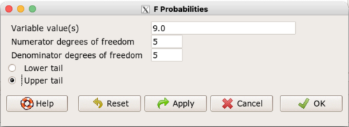
Figure 1. Screenshot R Commander F distribution probabilities.
This will return the p-value, and you would interpret this against your Type I error rate of 5% as you do for other tests.
From Table 2, Appendix – F distribution we find 
And the p-value = 0.015
pf(c(9), df1=5, df2=5, lower.tail=FALSE)
[1] 0.01537472
Question: Reject or Accept null hypothesis?
Question: What is the biological interpretation or conclusion from this result?
R code
Rather than play around with the tables of critical values, which are awkward and old-school (and I am showing you these stats tables so that you get a feel for the process, not so you’d actually use them in real practice), use Rcmdr to generate the F test and therefore return the F distribution probability value. As you may expect, R provides a number of options for testing the equal variances assumption, including the F test. The F test is limited to only two groups and, because it is a parametric test, it also makes the assumption of normality, so the F test should not be viewed as necessarily the best test for the equal variances assumption among groups. We present it here because it is a logical test to understand and because of its relevance to the Mean Square ratios in the ANOVA procedures.
So, without further justification, here is the presentation on how to get the F test in Rcmdr. At the end of this section I present a better procedure than the F test for evaluating the equal variance assumption called the Levene test.
Return to the bite data in the table above and enter the data into an R data frame. Note that the data in the table above are unstacked; R expects the data to be stacked, so either create a stacked worksheet and transcribe the data appropriately into the cells of the worksheet, or, go ahead and enter the values into two separate columns then use the Stack variables in active data set… command from the Data menu in Rcmdr.
Then, proceed to perform the F test.
Rcmdr: Statistics → Variances → Two variances F-test…
The first context menu popup is where you enter the variables (Fig 2).
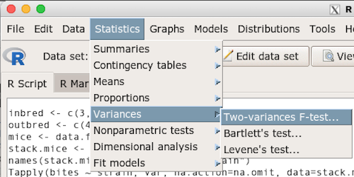
Figure 2. Screenshot data options R Commander F test
Because there are only two variables in the data set and because Strain contains the text labels of inbred or outbred whereas the other variable is numeric data type, R will correctly select the variables for you by default. Select the “Options” tab to set the parameters of the F test (Fig. 3).
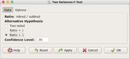
Figure 3. Screenshot menu options R Commander F test.
When you are finished setting the alternative hypothesis and confidence levels, proceed with the F test by clicking the OK button.
    F test to compare two variances

data:  mice.aggression
F = 0.1111, num df = 5, denom df = 5, p-value = 0.03075
alternative hypothesis: true ratio of variances is not equal to 1
95 percent confidence interval:
 0.01554788 0.79404243
sample estimates:
ratio of variances
         0.1111111
End of R output.
Levene’s test of equal variances
We will discuss this test in more detail following our presentation on ANOVA. For now, we note that the test works on two or more groups and is a conservative test of the equal variance assumption. Nonparametric tests in general make fewer assumptions about the data and in particular make no assumption of normality like the F test. It is in this context that the Levene’s test would be preferable over the F test. Below we present only how to calculate the statistic in R and Rcmdr and provide the output for the same mouse data set.
Assuming the data are stacked, obtain the Levene’s test in Rcmdr by clicking on (Fig 4).
Rcmdr: Statistics → Variances → Levene’s test…
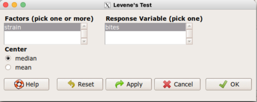
Figure 4. Screenshot menu options R Commander Levene’s test.
Select the median and the factor variable (in our case “Strain”) and the numeric outcome variable (“Bites”), then click OK button.
Tapply(bites ~ strain, var, na.action=na.omit, data=mice.aggression) # variances by group
inbred outbred
   0.8     7.2

leveneTest(bites ~ strain, data=mice.aggression, center="median")
Levene's Test for Homogeneity of Variance (center = median)
      Df F value  Pr(>F)
group  1       4 0.07339 .
      10
---
Signif. codes:  0 '***' 0.001 '**' 0.01 '*' 0.05 '.' 0.1 ' ' 1
End of R output
Compare the p-values. In both cases — F test and Levene’s test — we’re testing the same hypothesis (equal variances), but the p-values do not agree between the parametric F test and the nonparametric Levene’s test! If we were to go by the results of the F test, p-value was 0.031, less than out Type I error of 5% and we would tentatively conclude that the assumption of equal variances may not apply. On the other hand, if we go with the Levene’s test the p-value was 0.074, which is greater than our Type I error rate of 5% and we would therefore conclude the opposite, that the assumption of equal variances might apply! Both conclusions can’t hold, so which test result of equal variances do we prefer, the parametric F test or the nonparametric Levene’s test? Answer — we’d go with Levene’s because the F test is parametric and, therefore, also assumes normality.
Cahoy’s bootstrap method
Draft. Cahoy (2010). Variance-based statistic bootstrap test of heterogeneity of variances. we discuss bootstrap methods in Chapter 19.2; in brief, bootstrapping involves resampling the dataset and computing a statistic on each sample. This method may be more powerful, that is, more likely to correctly reject the null hypothesis when warranted, compared to Levene’s test.
for now, install package testequavar.
Function for testing two samples.
equa2vartest(inbred, outbred, 0.05, 999)
R output
[[1]]
[1] "Decision: Reject the Null"
$Alpha
[1] 0.05
$NumberOfBootSamples
[1] 999
$BootPvalue
[1] 0.006
The output “Decision: Reject the Null” reflects output from a box-type acceptance region.
Compare results from Levene’s test: p-value 0.07339 suggests accept hypothesis of equal variances, whereas bootstrap method indicates variances heterogenous, i.e., reject equal variance hypothesis. However, re-running the test without setting the seed for R’s pseudorandom number generator will result in different p-values. For example, I re-ran Cahoy’s test five times with the following results:
0.008
0.006
0.002
0.01
0.004
Questions
- Test assumption of equal variances by Bartlett’s method and by Levene’s test on
OliveMomentvariable from the Comet tea data set introduced in Chapter 12.1. Do the methods agree? If not, which test result would you choose?- BONUS. Retest homogeneous variance hypothesis by
equa3vartest(Copper.Hazel, Copper, Hazel, 0.05, 999). Reject or fail to reject the null hypothesis by bootstrap method?
- BONUS. Retest homogeneous variance hypothesis by
- Test assumption of equal variances by Bartlett’s method and by Levene’s test on
Heightfrom the O’hia data set introduced in Chapter 12.7. Do the methods agree? If not, which result would you choose?- BONUS. Retest homogeneous variance hypothesis by
equa3vartest(M.1, M.2, M.3, 0.05, 999). Reject or fail to reject the null hypothesis by bootstrap method?
- BONUS. Retest homogeneous variance hypothesis by
Quiz Chapter 13.4
Tests for Equal Variances
R code reminders
The bootstrap method expects the variables in unstacked format. A simple method to extract the variables from the stacked data is to use a command like the following. For example, extract OliveMoment values for Copper-Hazel treatment.
Copper.Hazel <- cometTea$OliveMoment[1:10]
For Copper, Hazel, replace above with [11:20], and [21-30] respectively. Note: changed variable name from Copper-Hazel to Copper.Hazel. The hyphen is a reserved character in R.