0.2 – List of figures
507 figures
updated 20 Feb 2026
1.1 – A quick look at R and R Commander
Figure 1. Choose how you will interact with R: on your computer (Blue box) or in the cloud (Red box). Users of Linux, macOS, and WinPC can also choose to access R in the cloud (black arrow).
Figure 2. R.app icon shown on a MacBook dock.
Figure 3. The R GUI on a macOS system; red arrow points to the R prompt.
Figure 4. Screenshot of drop down menu RGUI, create new script, Windows 10
Figure 5. Screenshot of portion of R Script editor, Windows 11. A simple R command is visible.
Figure 6. The windows of R Commander, macOS. From bottom to top: Messages, Output, Script (tab, Markdown) Rcmdr ver. 2.4-4.
Figure 7. The windows of R Commander, Win11. From bottom to top: Messages, Output, Script (tab, R Markdown) Rcmdr ver. 2.5-1.
Figure 8. Screenshot of terminal window (cmd) on win11 computer, checking for installed pandoc on a win10 pc.
Figure 9. Screenshot of GUI preferences settings after changing from default MDI to SDI, win10
Figure 10. Screenshot Rcmdr Tools popup menu, macOS 10.15.6
Figure 11. Screenshot Rcmdr Set app nap dialog box, macOS 10.15.6
2.2 – Why do we use R Software?
Figure 1. A basic workflow with R.
Figure 2. “Spreadsheets,” xkcd.com no. 2180
Figure 3. Basic scatter plot made in R, plot(A,B).
Figure 4. Basic scatterplot made in Microsoft Excel.
Figure 5. Basic scatterplot made in LibreOffice Calc.
2.3 – A brief history of (bio)statistics
Figure 1. Soldiers playing dice, painting by Michiel Sweerts (1618–1664). Public domain image, https://commons.wikimedia.org/
Figure 2. Original map by John Snow showing the clusters of cholera cases in the London epidemic of 1854, drawn and lithographed by Charles Cheffins. Image Public Domain, from Wikipedia
Figure 3. Plot of Snow’s London using R cholera package. Triangles marked with p1-p13 represent public water pumps. Red dots represent cholera cases.
Figure 4. Plot of Snow’s London with walking areas drawn about the 13 water pumps. R cholera package.
2.4 – Experimental Design and rise of statistics in medical research
Figure 1. Left: ASARCO smelter, Ruston, Washington, image from Department of Ecology, State of Washington. Direction of smoke from the stack is north, toward Vashon Island. Right: Heat map of arsenic and lead affected areas. image from kingcounty.gov. Darker regions correspond to heavier arsenic and lead contamination of soils.
Figure 2. County cancer rates (A, lung and bronchial; B, bladder) from 2000 – 2020 vs distance in kilometers from ASARCO smelter, Ruston, WA. Data compiled from Washington Tracking Network (WTN). The counties were King (55 km), Kitsap (39.28 km), Pierce (38.48 km), San Juan ( 141.43 km), Snohomish (100.73 km), and Spokane (385.34 km).
2.5 – Scientific method and where statistics fits
Figure 1. “Frequentists vs Bayesians,” xkcd.com no. 1132
Figure 2. Probability tree diagram with prevalence of type 2 diabetes and sensitivity, specificity of A1C test, data from CDC and Selvin et al 2011. Tree drawn with free diagrams.net app.
2.6 – Statistical reasoning
Figure 1. “Survivorship bias,” https://www.xkcd.com/1827/
Figure 2. “Selection bias,” https://xkcd.com/2618/
3.1 – Data types
Figure 1. Five Conus shells, example of discrete data type. Click image to view full sized image.
Figure 2. Analog thermometer showing office temperature at 23.1 Celsius, example of interval data type. Click image to view full sized image.
Figure 3. Blood glucose reading, 122 mg/dL. Click image to view full sized image.
Figure 4. Analog hygrometer showing office humidity at 65 percent, example of ratio data type. Click image to view full sized image.
Figure 5. Flowers (Hydrangea) are blue or they are not, example of binomial data type. Click image to view full sized image.
Figure 6. Cats are neither dogs or wolves, example of nominal data type. Click image to view full sized image.
Figure 7. Screenshot Rcmdr Read data from package menu.
3.2 – Measures of Central Tendency
Figure 1. A portion of the R help page about the function mean.
Figure 2. Dot plot of our x variable with locations of the mean (blue) and the trimmed mean (red). The Dotplot(x) function in package RcmdrMisc was used in Rcmdr to make this graphic. Arrows were added by hand. Dotplot() example code presented in Chapter 3.4.
Figure 3. Normal and lognormal distributions with mean (red) and median (blue) noted for comparison.
Figure 4. Histogram, box plot, and cumulative distribution function plot generated by default by Desc() call.
Figure 5. Screenshot R Commander, summary statistics by group.
Figure 6. Female Rhinella marina (formerly Bufo marinus), Chaminade. University campus. Body length 23.5 cm.
3.3 – Measures of dispersion
Figure 1. A histogram which displays a sampling of data with a mean of 10 (arrow marks the spot) and standard deviation (sd) of 50 units.
Figure 2. A histogram which displays a sampling of data with the same mean of 10 (arrow marks the spot) displayed in Fig. 1, but with a smaller standard deviation (sd) of 5 units.
Figure 3. Histogram of ages of subjects in the diabetic retinopathy data set in the survival package.
Figure 4. Scatter plot of the standard deviation (StDev) by the mean. Data sets were simulated.
Figure 5. Plot of the standard deviation by the mean for heights of different breeds of dogs.
3.4 – Estimating parameters
Figure 1. Dot plot of pipet results.
3.5 – Statistics of error
Figure 1. Magnetic dart board with 5 darts. Click image to view full sized image.
4 – How to report statistics
Figure 1. Scatter plot graphs of Anscombe’s quartet (Table 1)
Figure 2. Excel pie chart of Table 2 data set
Figure 3. Bar chart of Table 2 data set
4.1 – Bar (column) charts
Figure 1. Single nucleotide variants for human gene ACTB by DNA and functional element (data collected 19 May 2022 from NCBI SNP database with Advanced search query). A. Pie chart. Note that slide for “exon – nonsense” is not visible. B. Bar chart – color coded bars to facilitate comparison with pie chart.
Figure 2. A simple bar chart
Figure 3. The luxury ship RMS Titanic, which sunk 15 April 1912, More than 1500 souls were lost. Public domain image, Wikipedia. Click image to view full sized image.
Figure 4. A stacked bar chart, survival Titanic
Figure 5. A bar chart with error bars (standard error of the mean).
Figure 6. Another bar chart. with standard errors of mean
Figure 7. Bar chart that allows for a comparison among levels of a a factor (organs, liver vs. heart).
Figure 8. Same chart as in Figure 6, but on ratios.
Figure 9. Rcmdr menu popup for Plots Means
Figure 10. Plot of means
Figure 11. A bar chart using barplot2.
Figure 12. A barchart from ggplot2
4.2 – Histograms
Figure 1. Histograms of age distribution of runners who completed the 2103 Jamba Juice 5K race in Honolulu
Figure 2. KDE plot of age distribution of female runners who completed the 2103 Jamba Juice 5K race in Honolulu
Figure 3. Histogram of 752 observations, Sturge’s rule applied, default histogram
Figure 4. Histogram of 752 observations, Scott’s rule applied, ggplot2 histogram
Figure 5. Default histogram with different bin size
Figure 6. Default histogram, bin size set by Sturge’s rule.
Figure 7. Two histograms on same plot with ggplot2.
Figure 8. Same data as Fig 7, but using base hist() and plot() functions.
Figure 9. Using only base R graphics, a lot with region between 40 and 60 highlighted in red.
Figure 10. Using geom_ribbon() and ggplot2 package, a plot with region between 40 and 60 highlighted in red.
Figure 11. Examples of comet assay results.
4.3 – Box plot
Figure 1. A box plot. Elements of box plot labelled.
Figure 2A. Box plot, default graph in base package
Figure 2B. Same graph, but with color and made horizontal; boxplot(), default graph in base package
Figure 2C. Same graph, added original points; boxplot(), default graph in base package.
Figure 3. Popup menu in R Commander: Select the response variable and set the Plot by: option.
Figure 4. Select the group variable
Figure 5. Options tab, enter labels for axes and a title.
Figure 6. Resulting box plot from car package implemented in R Commander. Outliers are identified by row id number.
Figure 7. Screen shot of Load Rcmdr plug-ins menu, Click OK to proceed (see Fig 8).
Figure 8. To complete installation of the plug-in, restart R Commander.
Figure 9. Menu of KMggplot2. A title was added, all else remained set to defaults.
Figure 10. Default box plot from KMggplot.
Figure 11. “Economist” theme box plot from KMggplot2.
Figure 12. Tufte theme and data points added to the box plot.
4.4 – Mosaic plots
Figure 1. Mosaic plot made with basic function mosaicplot().
Figure 2. First steps to make mosaic plot in R Commander EBM plug-in.
Figure 3. Next steps to make mosaic plot in R Commander EBM plug-in.
Figure 4. Mosaic plot made from R Commander EBMplug-in
Figure 5. First steps to make mosaic plot in R Commander KMggplot2 plug-in
Figure 6. Next steps to make mosaic plot in R Commander KMggplot2 plug-in.
Figure 7. Mosaic-like plot made from R Commander KMggplot2 plug-in.
Figure 8. Screenshot of popup menu from Rcmdr with mosaic plugin selected.
Figure 9. After clicking OK (Fig 8), click Yes to restart Rcmdr. The plugin will then be available.
Figure 10. How to access the mosaic plot in R Commander.
Figure 11. Screenshot of popup menu in mosaic plugin in R Commander.
Figure 12. Error message as result of selecting a dataframe for use in mosaic plugin.
Figure 13. Options for the mosaic plot
Figure 14. Our new mosaic plot.
Figure 15. Mosaic plot with changed color scheme.
4.5 – Scatter plots
Figure 1. Scatterplot of mid-parent (vertical axis) and their adult children’s (horizontal axis) height, in inches. data from Galton’s 1885 paper, “Regression towards mediocrity in hereditary stature.” The red line is the linear regression fitted line, or “trend” line, which is interpreted in this case as the heritability of height
Figure 2. Same plot as Figure 1, but with default settings for axis scales.
Figure 3. Finishing times in minutes of 1278 runners by age and gender at the 2013 Jamba Juice Banana 5K in Honolulu, Hawaiʻi. Loess smoothing functions by groups of female (red) and male (blue) runners are plotted along with 95% confidence intervals.
Figure 4. First menu popup in R Commander Scatterplot command, Rcmdr ver. 2.2-3.
Figure 5. Second menu popup in R Commander scatterplot command., Rcmdr ver. 2.2-3
Figure 6. Default scatterplot, package car, from R Commander, version 2.2-4.
Figure 7. Modified scatterplot, same data from Figure 6
Figure 8. R plotting characters pch = 1 – 25 along with examples of color.
Figure 9. Usage of terms for X Y plots in research articles normalized to number of issues in six journals between 1990 and 2016.
Figure 10. Results from Ngram Viewer for American English, “scatterplot” (blue), “scatter plot” (red), “scatter diagram” (green), “scattergram” (orange), and “XY plot” (purple).
Figure 11. Results from Ngram Viewer for British English. See Figure 10 for key.
Figure 12. Bland-Altman plot of 1 cm unit measure in pixel number by imageJ from digital images by two independent observers. Purple central region is 95% CI.
Figure 13. Volcano plot, gene expression fold change (graph pending).
4.6 – Adding a second Y axis
Figure 1. Screenshot from NOAA GOES-East – Sector view: Tropical Atlantic – GeoColor, 4 September 2019. Click image to view full sized image.
Figure 2. Plot of hurricanes from 1900 to present by decade.
Figure 3. Total number of hurricanes by decades, with Temperature Index by decades. Number of hurricanes represented on first (left) axis and Temperature Index represented on second (right) axis.
Figure 4. Total number of hurricanes by decades, with Atmospheric CO2 measured at Mauna Kea by decades. Number of hurricanes represented on first (left) axis and Atmospheric CO2 represented on second (right) axis.
4.7 – Q-Q plot
Figure 1. A Q-Q plot, the default command in Rcmdr
Figure 2. Screenshot of R Commander menu for Q-Q plot
4.8 – Ternary plots
Figure 1. Blank Graphics window with initial ternary plot.
Figure 2. A few Skittles® candies.
Figure 3. Ternary plot of our Skittle critter data.
Figure 4. rs4988235 genotype frequencies, data.SNP.
4.9 – Heat maps
Figure 1. Heat map, USA population by county and percent ethnicity compared to white, graph from census.gov
Figure 2. Heat map, gene expression in cultured rat lung cells exposed to metals
Figure 3. A simple heat map generated by heatmap() function, all default options.
Figure 4. ggplot() and aes() functions used to generate a heat map. Colors from brewer.pal
4.10 – Graph software
Figure 1. Screenshot of GrapheR GUI menu, box plot options
Figure 2. Box plot made with GrapheR.
Figure 3. Screenshot of KMggplot2 GUI menu, box plot options
Figure 4. Box plot graph made with GrapheR with jitter applied to avoid overplotting of points.
Figure 5. Box plot graph made with GrapheR with beeswarm applied to avoid overplotting of points.
Figure 6. Screenshot of plotly box plot. Live version, data points visible when mouse pointer hover.
Figure 7. Screenshot of box plot example in Veusz GUI.
Figure 8. Screenshot SciDAVis app with default box plot.
5 – Experimental design
Figure 1. Giant African Snail (Lissachatina fulica, formerly Achatina fulica). Image by M. Dohm
5.2 – Experimental units, Sampling units
Figure 1. Plate layout for Table 1. Plot made with plate_plot() function from R package ggplate.
Figure 2. Three aquariums, three fish. Image modified from https://www.pngrepo.com/svg/153528/aquarium
Figure 3. Three Miracle-Grow AeroGarden planters, each with nine seedlings of an Arabidopsis thaliana strain.
5.3 – Replication, Bias, and Nuisance Variables
Figure 1. Schematics of a set up for a hypothetical 48 well microplate (plate_plot() from ggplate package).
Figure 2. Mean 5K running times (minutes) by age and gender (2006 – 2016, Jamba Juice Banana 5K race, Honolulu, HI).
5.4 – Clinical trials
Figure 1. Search of PUBMED for “RCT” and “double blind” studies from 1950 to 2024.
5.5 – Importance of randomization in experimental design
Figure 1. Age of subjects by groups (A = blue, B = red) with and without randomized assignment of subjects to treatment groups
Figure 2. BMI of subjects by groups (A = blue, B = red) with and without randomized assignment of subjects to treatment groups
Figure 3. An example of clustering resulting from a random sampling process (Graph B). In contrast, Graph A was generated so that a point was located within each grid.
Figure 4. Same graphs as Figure 3, but with ellipses around the grouped data (hard to tell, but the centroids are the larger points).
Figure 5. Map of electrical transmission grid for continental United States of America. Image source https://openinframap.org/#3/24.61/-101.16
5.6 – Sampling from Populations
Figure 1. Sixteen mice, eight red and eight blue. Image © 2024 Mia D Graphics
Figure 2. Sixteen mice, randomly assigned to treatment groups C and T; by chance, 75% blue in C and just 25% in T. If color was a confounding factor then our conclusions about the effectiveness of the treatment would be associated with color. Image © 2024 Mia D Graphics
Figure 3. Format of 96-well plate. Red cells = “edge” wells; White cells = “inner” wells; Well reference in grey letter.
Figure 4. Screenshot of Sampling in Data Analysis menu, Microsoft Excel
Figure 5. Screenshot of input required for Sampling in Data Analysis menu, Microsoft Excel
6.1 – Some preliminaries
Figure 1. Slides,” https://xkcd.com/365/ .
Figure 2. View of Kamokuna Lava Bench, eruption of Pu`u `O`o, Kilauea, November 1998. Photo by S. Dohm.
Figure 3. Mark Twain. Image from The Miriam and Ira D. Wallach Division of Art, Prints and Photographs: Photography Collection, The New York Public Library. “Mark Twain in Middle Life” The New York Public Library Digital Collections. 1860 – 1920. https://digitalcollections.nypl.org/items/510d47d9-baec-a3d9-e040-e00a18064a99
Figure 4. “Hand sanitizer,” https://imgs.xkcd.com/comics/hand_sanitizer.png.
6.2 – Ratios and probabilities
Figure 1. Example planting of five tomato seeds, day 5, on agar Petri dish (M. Dohm)
Figure 2. A probability tree to help visualize comparison of deaths (“yes”) by car travel and by airline travel in the United States for the year 2000.
Figure 3. Comparing totals of deaths adjusted by numbers of licensed drivers and by licensed commercial airline pilots in the United States.
Figure 4. Comparing totals of deaths adjusted by numbers of car trips and by numbers of airline trips in the United States.
6.3 – Combinations and permutations
Figure 1. Heads (left) and Tails (right) of a Susan B. Anthony dollar.
Figure 2. Playing cards with images commemorating 150th anniversary of Charles Darwin’s Origin of Species. (Design John R. C. White, Master of the Worshipful Company of Makers of Playing Cards 2008 to 2009.)
Figure 3. Bar chart of the combinations of correct guesses out of 10 attempts (graph was presented in Chapter 4.1).
6.5 – Discrete probability distributions
Figure 1. Plot generated with KMggplot2 Rcmdr plugin.
Figure 2. Example of binomial-like distribution: reported twin births, Hawaiʻi.
Figure 3. Rcmdr menu to get binomial probability.
Figure 4. Plot of hypergeometric distribution twinning Hawaiʻi.
Figure 5. Rcmdr menu to get hypergeometric probability.
Figure 6. Example, poisson-like graph: the number of wind-dispersed seeds within each grid.
Figure 7. The probability of observing a grid with five seeds, poisson μ = 1 (ggplot2).
Figure 8. Rcmdr menu, poisson probability.
6.6 – Continuous distributions
Figure 1. Sample size = 20, drawn from population with known μ = 0 and σ = 1.
Figure 2. Sample size = 100, also drawn from population with known μ = 0 and σ = 1.
Figure 3. Sample size n = 1000, once again drawn from population with known μ = 0 and σ = 1.
Figure 4. And lastly, sample size n = 1 million also drawn from population with known μ = 0 and σ = 1.
Figure 5. Screenshot Rcmdr menu, sample from a normal distribution.
Figure 6. Frequency expected for a few points (X: 0 – 10) drawn from a normal distribution, calculated using the formula and example values.
6.7 – Normal distribution and the normal deviate (Z)
Figure 1. Frequency of observations expected to be greater than 7 from a large population with mean µ = 5 and σ = 2.
Figure 2. Portion of the table of the normal distribution. Only values equal to or greater than Z = 0 are visible.
Figure 3. Highlight Z = 0.23, frequency is 0.409046.
Figure 4. Plot of standard normal distribution; area less than -1 σ.
Figure 5. proportion of the population is between 5 and 7.
6.8 – Moments
Figure 1. Histogram finishing times in minutes for 1307 runners at 2016 Banana 5K.
Figure 2. Rcmdr Numerical summaries Statistics tab.
Figure 3. Histogram finishing times in minutes for random sample of 30 drawn from 1307 runners at 2016 Banana 5K.
Figure 4. Screenshot Rcmdr menu: Sample from Chisquare distribution.
6.9 – Chi-square distribution
Figure 1. Animated GIF of plots of chi-square distribution over range of degrees of freedom.
Figure 2. The test of the chi-square is typically one-tailed. In this case, probability of values greater than the critical value.
Figure 3. Portion of the table of some critical values of chi-square distribution, one tailed (right-tailed or “upper” portion of distribution).
Figure 4. Portion of the chi-square distribution which shows how to find critical value of the chi-square distribution.
Figure 5. Screenshot of input box in Rcmdr for Chi-square probability values.
6.10 – t distribution
Figure 1. Density plot of standard normal distribution.
Figure 2. Density plot of t-distribution for five degrees of freedom.
Figure 3. Animated GIF of density plot t distribution, from df = 5 to 10,000 plus standard normal curve.
6.11 – F distribution
Figure 1. Animated GIF plot of F distribution value for range of degrees of freedom.
7 – Probability, Risk Analysis
Figure 1. “Health data,” https://xkcd.com/2620/.
7.2 – Epidemiology basics
Figure 1. R Commander popup menu for Normal quantiles.
7.3 – Conditional Probability and Evidence Based Medicine
Figure 1. Now that’s a box full of kittens. Creative Commons License, source: https://www.flickr.com/photos/83014408@N00/160490011.
Figure 2. STS-51-L crew: (front row) Michael J. Smith, Dick Scobee, Ronald McNair; (back row) Ellison Onizuka, Christa McAuliffe, Gregory Jarvis, Judith Resnik. Image by NASA – NASA Human Space Flight Gallery, Public Domain.
Figure 3. Space Shuttle Challenger launches from launchpad 39B Kennedy Space Center, FL, at the start of STS-51-L. Hundreds of shorebirds in flight. Image by NASA – NASA Human Space Flight Gallery, Public Domain.
Figure 4. Probability tree for FOBT test; Good test outcomes shown in green: TP stands for true positive and TN stands for true negative. Poor outcomes of a test shown in red: FN stands for false negative and FP stands for false positive.
Figure 5. A summary of “evidence based medical” decisions, perhaps? “Watson Medical Algorithm,” https://xkcd.com/1619/.
Figure 6. To install an Rcmdr plugin, first go to Rcmdr → Tools → Load Rcmdr plug-in(s)…
Figure 7. Select the Rcmdr plugin, then click the “OK” button to proceed.
Figure 8. Select “Yes” to restart R Commander and finish installation of the plug-in.
Figure 9. After restart of R Commander the EBM plug-in is now visible in the menu.
Figure 10. Select “Enter two-way table…”.
Figure 11. Two-way table Rcmdr EBM plug-in.
Figure 12. Draw a probability tree to help with the frequencies.
Figure 13. EBM plugin with data entry.
7.4 – Epidemiology: Relative risk and absolute risk, explained
Figure 1. Data entry for 2X2 table at openepi.com.
Figure 2. Results for 2X2 table at openepi.com.
Figure 3. Rcmdr: Tools → Load Rcmdr plugins…
Figure 4. Rcmdr plug-ins available (after first download the files from an R mirror site).
Figure 5. R Commander EBM plug-in, enter 2X2 table menus.
Figure 6. Illustration of probability tree for the statin problem.
Figure 7. EBM plugin with two-way table completed for the statin problem.
7.5 – Odds ratio
Figure 1. Mosaic plot of athletes to non-athletes in college. Males red, females yellow, data from Gray 2002
Figure 2. Venn Diagram of athletes to non-athletes in college. Female athletes (n = 375), male athletes (n = 612), data from Gray 2002.
8 – Inferential statistics
Figure 1. NHST decision flow chart.
8.1 – The null and alternative hypotheses
Figure 1. Flow chart of inductive statistical reasoning.
8.2 – The controversy over proper hypothesis testing
Figure 1. Screenshot t-quantiles Rcmdr menu.
Figure 2. Screenshot of portion of t-table with highlighted (red) critical value for 10 degrees of freedom.
Figure 3. “Frequentists vs. Bayesians,” https://xkcd.com/1132/.
Figure 4. Conditional error probability values plotted against p-values.
8.3 – Sampling distribution and hypothesis testing
Figure 1. means of ten replicate samples drawn at random from chi-square distribution, df = 1.
Figure 2. means of 100 replicate samples drawn at random from chi-square distribution, df = 1. Results from Shapiro-Wilks test: W = 0.97426, p-value = 0.04721.
Figure 3. means of one million replicate samples drawn at random from chi-square distribution, df = 1. Normality test will fail to run, sample size of 5000 limit.
Figure 5. Screenshot Rcmdr menu to get normal probability.
8.4 – Tails of a test
Figure 1. Two-tailed distribution.
Figure 2. One-tailed distribution, lower tail (left) and upper tail (right).
8.5 – One sample t-test
Figure 1. Table of a portion of the Critical values of the t distribution. Red selections highlight critical value for t-test at α = 5% and df = 19.
Figure 2. Screenshot Rcmdr single-sample t-test menu.
9.1 – Chi-square test: Goodness of fit
Figure 1. A portion of critical values of the chi-square at alpha 5% for degrees of freedom between 1 and 10. A more inclusive table is provided in the Appendix, Table of Chi-square critical values.
Figure 2. R Commander menu for Chi-squared quantiles.
Figure 3. R Commander menu for Chi-squared probabilities.
9.2 – Chi-square contingency tables
Figure 1. Screenshot R Commander menu for 2X2 data entry with counts.
Figure 2. Display of Xiang et al data entered into R Commander menu.
Figure 3. Screenshot Statistics options for contingency table.
9.5 – Fisher exact test
Figure 1. Screenshot Rcmdr menu, Contingency tables.
Figure 2. Screenshot Rcmdr menu, Enter Two-Way Table.
Figure 3. Screenshot Rcmdr two-way table menu, load the data from stacked worksheet.
Figure 4. Screenshot Rcmdr menu Statistics option. Select Chi-square test of independence, Fisher’s exact test, or both.
10.1 – Compare two independent sample means
Figure 1. A two group Randomized Control Trial.
Figure 2. Male Hemidactylus frenatus, central Oahu, M. Dohm.
Figure 3. Male Anolis carolinensis, `Akaka Falls, Big Island of Hawaiʻi, M. Dohm.
Figure 4. Box plot of lizard body mass.
Figure 5. Rcmdr menu for Independent sample t-test.
Figure 6. Rcmdr Options menu for Independent sample t-test.
Figure 7. Comet examples. A Intact cell, no DNA damage, B Cell with some DNA damage, a slight tail to the right is evident, C Cell with significant DNA damage, a large tail is evident. M. Dohm.
Figure 8. Boxplot of comet tail lengths for cells with and without (control) exposure to copper in the cell medium for 30 minutes.
10.2 – Digging deeper into t-test Plus the Welch test
Figure 1. Screenshot Rcmdr t-test options. Default is “No” for Assume equal variances, i.e., the Welch test.
10.3 – Paired t-test
Figure 1. A two group Randomized Crossover Trial.
Figure 2. Histograms shows the distribution of 5K running times of 15 women who ran the race twice.
Figure 3. Box plot of race speed (kph) for 15 women 5K in two successive years.
Figure 4. Profile plot, PairedData package.
Figure 5. Box plot of differences, Red dotted lines shows the null hypothesis.
Figure 6. R Commander Paired t-test menu, Rcmdr version 2.7.
Figure 7. R Commander Paired t-Test options, select null hypothesis.
Figure 8. R Commander: Stack worksheet. Select the two variables, Race1 and Race2.
Figure 9. R Commander, select independent sample t-Test …
Figure 10. R commander, independent sample t test menu.
Figure 11. R Commander, select options for independent sample t-Test (assume equal variance).
11.1 – What is Statistical Power?
Figure 1. Population sampling from tail of distribution.
Figure 2. Without us knowing, our sample may come from the extremes of two separate populations.
11.5 – Power analysis in R
Figure 1. Screenshot of Rcmdr menu bar with (A) and without (B) the EZR plugin.
Figure 2. Screenshot of Rcmdr EZR plugin menu.
Figure 3. Screenshot of EZR Menu to obtain sample size for the comparison between two (sample) means.
12.2 – One way ANOVA
Figure 1. Hypothetical results of an experiment, box plots. Left, no difference among groups; Right, large differences among groups.
Figure 2. Screenshot Rcmdr select one-way ANOVA.
Figure 3. Screenshot Rcmdr select one-way ANOVA options.
Figure 4. Box plot of lengths of leaves of a 10-day old plant from on of three strains of Arabidopsis thaliana.
12.3 – Fixed effects, random effects, and agreement
Figure 1. Honolulu Marathon 2024 participant. Image credit: Pdubs.94, licensed under CC BY 4.0 (Creative Commons Attribution 4.0 International License), via Wikipedia.
Figure 2. View west along Interstate H-1 (Lunalilo Freeway) at 6AM, Honolulu, Oahu, Hawaii. Image used with permission, credit: S. Dohm.
Figure 3. Simple waterfall plot of race improvement for Table 3 data. Dashed horizontal line at zero.
Figure 4. A spaghetti plot of average commute speeds from Table 2 data.
Figure 5. A parallel coordinates plot of average commute speeds from Table 2 data.
Figure 6. A heat map of the commute speeds data set.
Figure 7. Conus shells, image by M. Dohm.
12.6 – ANOVA posthoc tests
Figure 1. One-way ANOVA menu in R Commander.
Figure 2. Screenshot Rcmdr menu: Select Tukey posthoc tests with the one-way ANOVA.
Figure 3. Plot of confidence intervals of Tukey HSD.
12.7 – Many tests one model
Figure 1. O’hia, Metrosideros polymorpha. Public domain image from Wikipedia.
Figure 2. The o`hia dataset as viewed in R Commander.
Figure 3. Box plots of growth responses of o`hia seedlings collected from three Maui sites, M-1 (elevation 750 ft), M-2 (elevation 1100 ft), and M-3 (elevation 6600 ft). Data adapted from Table 5 of Corn and Hiersey 1973.
Figure 4. R Commander, select to fit a Linear model.
Figure 5. Input linear model formula, Height ~ Site.
Figure 6. To retrieve an ANOVA table, select Models, Hypothesis tests, then ANOVA table…
Figure 7. Options for types of tests.
13.1 – ANOVA Assumptions
Figure 1. xkcd.com “Statistics,” https://xkcd.com/2400/.
Figure 2. Histogram of body mass (g) for 24 mammals (data from Boddy et al 2012).
Figure 3. Histogram of log10-transformed body mass observations from Figure 2.
Figure 4. Plot of brain and body weights (A) and log10-log10 transform (B) for a variety of species (data from Boddy et al 2012). The ratio is called encephalization index.
Figure 5. Q-Q plot, body mass, raw data. Compare to Figure 2.
Figure 6. Q-Q plot same data, log10-transformed, compare to Figure 3.
Figure 7. Phylogenetic tree of 24 species used in this report.
13.2 – Why tests of assumption are important
Figure 1. Screenshot of Rcmdr options menu for independent t-test. Red arrow points to default option “No,” which corresponds to Welch’s test.
13.3 – Test assumption of normality
Figure 1. Rattle descriptive graphics on Comet Copper dataset. Dotted line (top image) and red line (bottom image) follow the combined observations regardless of treatment.
Figure 2. Graphs describing different distributions. From top to bottom: Leptokurtosis, platykurtosis, negative skew, positive skew.
Figure 3. Histogram of simulated normal dataset, μ = 125, σ = 10.
Figure 4. Cumulated frequency of simulated normal dataset, μ = 125, σ = 10.
Figure 5. Histogram of simulated normal dataset, μ = 0, σ = 1.
Figure 6. Cumulated frequency of simulated normal dataset, μ = 0, σ = 1.
13.4 – Tests for equal variance
Figure 1. Screenshot R Commander F distribution probabilities
Figure 2. Screenshot data options R Commander F test.
Figure 3. Screenshot menu options R Commander F test.
Figure 4. Screenshot menu options R Commander Levene’s test.
14.1 – Crossed, balanced, fully replicated designs
Figure 1A. One of several possible outcome of two treatments (factors). A clear interaction: First Diet level population 1 has greatest weight change, whereas for second diet level, population 2 has greatest weight change.
Figure 1B. One of several possible outcome of two treatments (factors). Clearly, no interaction: Population 1 always lower response than Population 2 regardless of Diet.
Figure 2. Plots of the main effects for Diet factor, levels A and B, and Population, levels 1 and 2.
Figure 3. Interaction plot between two factors, Diet and Population.
Figure 4. Linear model menu in Rcmdr.
Figure 5. A plot showing no interaction between factor A and factor B for some ratio scale response variable.
14.2 – Sources of variation
Figure 1. ANOVA table for two-way, balanced, replicated design.
14.3 – Fixed effects, Random effects
Figure 1. Interaction example. At density D1, genotype 2 (red line) has higher growth rate; at density D2, the ranking switches: now, genotype 1 (black line) has higher growth rate.
Figure 2. Interaction example expanded for multiple genotypes over multiple densities.
14.4 – Randomized block design
Figure 1. Screenshot Rcmdr Linear Model menu.
Figure 2. Line graph of data presented in Table 2.
Figure 3. Juvenile garter snake, image from GetArchive, public domain.
14.7 – Rcmdr Multiway ANOVA
Figure 1. Screenshot Rcmdr multi-way ANOVA.
Figure 2. Predictor effect plots, Diet and Population on Response variable.
Figure 3. Screenshot Rcmdr linear model menu.
14.8 – More on the linear model in Rcmdr
Figure 1. Linear model menu in Rcmdr, version 2.7.0
Figure 2. Menu of linear model with repeat measures model, Rcmdr, version 2.7.0.
Figure 3. Rcmdr: Models → Hypothesis tests → ANOVA table… Rcmdr, version 2.7.0
Figure 4. Crossed, balanced design. Linear model menu, Rcmdr, version 1.9.2
Figure 5. Nested design, linear model menu, Rcmdr, version 1.9.2
15.1 – Kruskal-Wallis and ANOVA by ranks
Figure 1. Screenshot Rcmdr menu create new variable.
15.2 – Wilcoxon Rank Sum Test
Figure 1. Female common house gecko, Hemidactylus frenatus, central Oahu, M. Dohm 2018.
Figure 2. Male Anolis carolinensis, ʻAkaka Falls, Hawaiʻi, M. Dohm 2018.
Figure 3. Screenshot Rcmdr menu 2 sample Wilcoxon test. Options are selected by clicking on “Options” tab (see Fig. 4)
Figure 4. Screenshot of options tab Rcmdr menu 2 sample Wilcoxon test. Keep defaults to run the “Wilcoxon test.”
Figure 5. Screenshot of Rcmdr menu. Note Two- sample Wilcoxon test… not available.
15.3 – Wilcoxon signed rank test
Figure 1. R Commander paired Wilcoxon test menu (aka Wilcoxon signed rank sum test). Rcmdr version 2.7.
Figure 2. R Commander Options, select null hypothesis.
16 – Correlation, Similarity, and Distance
Figure 1. Bar chart with error bars
Figure 2. Box plots
Figure 3. Scatterplot with groups
16.1 – Product moment correlation
Figure 1. Scatterplot of Drosophila wing area by wing length
16.2 – Causation and Partial correlation
Figure 1. Unmeasured confounding variables influence association between independent and dependent variables, the characters or traits we are interested in.
Figure 2. Running times over 100 meters of top athletes since the 1920s.
Figure 3. Scatterplot birth weight by lead exposure.
Figure 4. Screenshot Rcmdr partial correlation menu
Figure 5. Trellis plot, correlations among variables.
Figure 6. Causal paths among variables.
16.3 – Data aggregation and correlation
Figure 1. Scatterplot crime rates of cities by number of Catholic churches
Figure 2. scatterplot crime rates of cities by number of secular humanist associations.
Figure 3. Illustration of ecological fallacy: positive association at level of groups (boxes, solid blue line), but negative association at level of individuals (black circles, red dashed lines).
Figure 4. Bubble plot of data used to make Figure 1. Plot by LibreOffice Calc.
Figure 5. Bubble plot of data used to make Figure 2. Plot by ggplot2 package in R.
16.4 – Spearman and other correlations
Figure 1. Drosophila wing area (mm2) by wing length (mm).
16.6 – Similarity and Distance
Figure 1. Cartesian plot of two points, the first at x1 = 1 and y1 = 1 and the second at x2 = 4 and y2 = 4.
Figure 2. RAPD gel (simulated) five kinds of beans.
17.1 – Simple linear regression
Figure 1. R commander menu interface for linear model.
Figure 2. Number of matings by body mass (g) of the male bird.
Figure 3. Same data as in Fig. 2, but with the “best fit” line.
Figure 4. Figure 3 redrawn to extend the line to the Y intercept.
Figure 5. 95% confidence interval about the best fit line.
17.4 – OLS, RMA, and smoothing functions
Figure 1. CO2 in parts per million (ppm) plotted by year from 1958 to 2014
Figure 2. Plot of ppm CO2 by month for the year 2013.
Figure 3. Plot with different smoothing values (0.5 to 10.0).
17.5 – Testing regression coefficients
Figure 1. Scatterplot of hypothetical x,y data for which the researcher may obtain a statistically significant linear fit to sample of data from population in which null hypothesis is true relationship between x and y.
Figure 2. Screenshot linear regression menu. More than explanatory (predictor or independent) variables may be selected, but only one response (dependent) variable may be selected.
Figure 3. Pearson Scott Foresman, Public domain, via Wikimedia Commons
Figure 4. Scatterplot of oxygen consumption by tadpoles (blue: Gosner developmental stage I [35 – 38]; red: Gosner developmental stage II [39 – 44]), vs body mass (g).
Figure 5. Boxplot of oxygen consumption by Gosner developmental stages (blue: stage I; red: stage 2).
17.6 – ANCOVA – analysis of covariance
Figure 1. Scatterplot of oxygen consumption by R. pipiens tadpoles vs body mass (g) by developmental group (Gosner stages I or II).
Figure 2. Copy of Figure 4, Chapter 17.5; boxplot of oxygen consumption of R. pipiens tadpoles by Gosner developmental stages.
Figure 3. Scatterplot with best-fit regression lines of \dot{V} O_{2} by \text{Body.mass} for Gosner State I (closed circle, solid line) and Gosner Stage II (open circle, dashed line) R. pipiens tadpoles.
17.8 – Assumptions and model diagnostics for Simple Linear Regression
Figure 1. An ideal plot of residuals
Figure 2. We have a problem. Residual plot shows unequal variance (aka heteroscedasticity).
Figure 3. Problem. Residual plot shows systematic trend.
Figure 4. Problem. Residual plot shows nonlinear trend.
Figure 5. Basic diagnostic plots. A: residual plot; B: Q-Q plot of residuals; C: Scale-location (aka spread-location) plot; D: leverage residual plot.
18 – Multiple Linear Regression
Figure 1. Growth of bacteria over time (optical density at 600 nm UV spectrophotometer) , fit by logistic function (dashed line).
18.1 – Multiple Linear Regression
Figure 1. Screenshot of Rcmdr linear model menu with our model elements in place.
Figure 2. Scatter plot of predicted LDL against dose of a statin drug. Regression lines represent the different statin drugs (Statin1, Statin2).
Figure 3. 3D plot of BMI and dose of Statin drugs on change in LDL levels (green Statin2, blue Statin1).
Figure 4. An example of a possible interactive 3D plot; the file embedded in this page is not interactive, just an animation.
Figure 5. R’s default regression diagnostic plots.
18.2 – Nonlinear regression
Figure 1. Ideal plot of residuals against values of X, the predictor variable, for a well-supported linear model fit to the data.
Figure 2. Example of residual plot; pattern suggests nonlinear fit.
Figure 3. Residual plot
Figure 4. Lifespan of 1881 mice from 31 inbred strains (Data from Yuan et al (2012) available at https://phenome.jax.org/projects/Yuan2.
Figure 5. Screenshot Rcmdr GLM menu. For logistic on ratio-scale dependent variable, select gaussian family and identity link function.
18.3 – Logistic regression
Figure 1. Lifespan of 1881 mice from 31 inbred strains (Data from Yuan et al [2012] available at https://phenome.jax.org/projects/Yuan2. Note: I labeled Y axis labeled “Survival Probability”; “Inverse Survival Probability” would be more accurate.
Figure 2. Access Generalized Linear Model via R Commander
Figure 3. Screenshot Rcmdr GLM menu. For logistic on ratio-scale dependent variable, select gaussian family and identity link function.
18.4 – Generalized Linear Squares
Figure 1. Box plot of residuals from GLS model by elevation site predictors (left) and scatterplot of residuals by fitted values from GLS model (right).
18.5 – Selecting the best model
Figure 1. Rcmdr popup menu, Subset model selection…
Figure 2. Mallow’s Cp plot
Figure 3. Diagnostic plots
18.6 – Compare two linear models
Figure 1. Screenshot Rcmdr compare models menu.
19.1 – Jackknife sampling
Figure 1. histogram of jackknife estimates for slope
Figure 2. Histogram of jackknife estimates for intercept.
19.2 – Bootstrap sampling
Figure 1. histogram of bootstrap estimates for slope
Figure 2. Histogram of bootstrap estimates for intercept.
19.3 — Monte Carlo methods
Figure 1. Histograms of runif results with 100, 1K, 10K, and 100K numbers of values to be generated
Figure 2. Autocorrelation plots of runif results with 100, 1K, 10K, and 100K numbers of values
20.1 – Area under the curve
Figure 1. Area under the curve example.
Figure 2. Example ROC curve
20.3 – Baseline correction
Figure 1. Simulated myogram data with baseline drift.
Figure 2. Simulated myogram data with random walk noise and baseline drift.
20.5 – Time series
Figure 1. co2 data set from package datasets, comes with Rcmdr installation.
Figure 2. CO2 ppm monthly average data from NOAA, last data October 2020.
Figure 3. Observed (panel, top), trends over time (panel, second from top), seasonal changes (panel, second from bottom), and random error (panel, bottom).
Figure 4. Data in black, predicted values in red (additive) shaded by confidence interval.
20.6 – Dimensional analysis
Figure 1. Scatterplot English swallow mass (g) by total length (mm) by survival following winter storm
Figure 2. Scatterplot matrix of Bumpus English sparrow traits. Traits were (left-right): Alar extent (mm), length (tip of beak to tip of tail), length of head (mm), length of femur (in.), length of humerus (in.), length of sternum (in.), skull width (in.), length of tibio-taurus (in.), and weight (g)
Figure 3. Bi-plot of clusters, Skittles mini bags
20.8 – Diversity indexes
Figure 1. (A) Chaminade University, a portion of lower campus; (B) A portion of Lyon Arboretum; (C) Portion of Roundtop Forest Reserve. Google satellite images, approximately the same altitude and sized areas.
20.9 – Survival analysis
Figure 1. Screenshot of menu call for survival analysis in Rcmdr
Figure 2. Kaplan-Meier plot of heart data. Dashed lines are upper and lower confidence intervals about the survival function.
Figure 3. KM plot
Figure 4. Screenshot of Survival estimator menu in Rcmdr.
20.10 – Growth equations and dose response calculations
Figure 1. Top: Parametric Nonlinear Growth Model; Bottom: Nonparametric Spline Fit
Figure 2. Hypothetical data set, survival of yeast in different salt concentrations.
Figure 3. Logistic curve added to Figure 1 plot.
Figure 4. Four parameter (red) and three parameter (green) logistic models fitted to data.
Figure 5. Plot of reduced data set.
Figure 6. Screenshot Microsoft Excel worksheet containing our data set (col A & B), with formulas added and calculated. Starting values for constants in column G, rows 2 – 4.
Figure 7. Screenshot Microsoft Excel, Solver add-in available.
Figure 8. Screenshot Microsoft Excel, Solver add-in available and ready for use.
Figure 9. Screenshot Microsoft Excel solver menu.
Figure 10. Screenshot solver completed run.
20.11 – Plot a Newick tree
Figure 1. Phylogram plot of 14 taxa
Figure 2. Cladogram view, same 14 taxa.
Figure 3. Plot of tree with labeled nodes.
Figure 4. Re-rooted tree.
Figure 5. Star phylogeny
20.12 – Phylogenetically independent contrasts
Figure 1. Star phylogeny (same image shown Figure 5, 20.11 – Plot a Newick tree).
Figure 2. A cladogram for same species, showing the hierarchical, nested relationships among taxa, what nature actually provides (same image shown Figure 2, 20.11 – Plot a Newick tree).
20.13 – How to get the distances from a distance tree
Figure 1. A gene tree of the product (protein HBA1) with five species.
Figure 2. Scatterplot HBA distance by logMYA divergence time.
20.15 – Meta-analysis
Figure 1. Forest plot, Cohen’s effect size lifespan differences among inbred strains of mice compared to outbred strain.
Appendix
Figure 1. Table for Z in the area under the standard normal curve to the right of the vertical line (area shaded blue).
Figure 2. Right-tail probability (> Χ2) chi-square critical value (area shaded blue).
Figure 3. Right-tail probability (> t) Student’s t distribution critical value (area shaded blue).
Figure 4. Right-tail probability (> F) F distribution critical value, df1,1 (area shaded blue).
Install R
Figure 1. Suggested flow chart for R installation.
Figure 2. Screenshot homepage for R-project.org.
Figure 3. Screenshot of portion of R-Project CRAN mirror page.
Figure 4. Screenshot of portion of base R download page.
Figure 5. Screenshot of RGui.exe (1), script editor (2), and results of plot() (3) on WinPC.
Figure 6. Screenshot of R.app (1), script editor (2), and results of plot() (3) on macOS.
Figure 7. Screenshot of RStudio IDE.
Figure 8. Screenshot RStudio desktop download page, current as of September 2025.
Figure 9. Screenshot — Find the R install file in your download folder.
Figure 10. Screenshot: first instructions pop-up window.
Figure 11. Screenshot: second instructions pop-up window.
Figure 12. Screenshot: third instructions pop-up window.
Figure 13. Screenshot: fourth instructions pop-up window.
Figure 14. Screenshot: fifth instructions pop-up window.
Figure 15. Screenshot: sixth instructions pop-up window.
Figure 16. Screenshot: seventh instructions pop-up window.
Figure 17. Screenshot: eighth and final instructions pop-up window.
Figure 18. Screenshot: MacOS will prompt with option to delete the installation file. This has no effect on the installation of R.
Figure 19. Screenshot: R Console in the R.app on macOS.
Figure 20. WinPC screenshot: Pop-up menu after right-click on the R installation file in windows Explorer.
Figure 21. WinPC screenshot: first instructions pop-up window.
Figure 22. WinPC screenshot: second instructions pop-up window.
Figure 23. WinPC screenshot: third instructions pop-up window. Note — R-4.5.1 (current version as of August 2025).
Figure 24. WinPC screenshot: fourth instructions pop-up window.
Figure 25. WinPC screenshot: fifth instructions pop-up window. Recommend setting to SDI.
Figure 26. WinPC screenshot: sixth instructions pop-up window.
Figure 27. WinPC screenshot: seventh instructions pop-up window.
Figure 28. WinPC screenshot: eighth instructions pop-up window.
Figure 29. WinPC screenshot: ninth instructions pop-up window.
Figure 30. WinPC screenshot: final instructions pop-up window — successful installation.
Install R Commander
Figure 1. Screenshot of basic R Commander session on WinPC.
Figure 2. Screenshot of portion of RcmdrMarkdown.pdf.
Figure 3. Screenshot of basic R Commander session in RStudio on macOS.
Use R in the cloud
Figure 1. Screenshot of myCompiler session.
Figure 2. Screenshot of CoCalc session.
Figure 3. Screenshot of Google Colab session.
Figure 4. QR code with url to create new R notebook in CoLab.
Figure 5. Screenshot of “Complete the Google auth process” page.
Figure 6. Screenshot, confirm R is the programming language in use by the Google Colab session.
Figure 7. Screenshot magic function rpy2 in action on CoLab, python environment.
Figure 8. Screenshot of RStudio at Posit Cloud session.
Figure 9. Screenshot of rdrr.io/snippets session.
Juputer Notebook
Figure 1. Screenshot of macOS terminal with command to start Jupyter lab.
Figure 2. Screenshot of Jupyter Lab. Select R icon under Notebook to set IRkernel.
Figure 3. Screenshot of Jupyter Notebook running the IRkernel.
Figure 4. Screenshot of Jupyter Console running R.
Figure 5. Screenshot of Notebook with Python set as kernel.
Figure 6. Screenshot of select kernel popup menu.
Figure 7. Screenshot of installed kernels.
Figure 8. Screenshot Jupyter Notebook, confirm R runtime is set (green circle).
Jupyter notebook
Draft
Introduction
Jupyter notebook, python. A “web-based computational environment”
Project homepage: https://jupyter.org/
Besides the python kernel, Jupyter kernels include
Cytoscape
SageMATH
and, of course R, which along with python and Julia, is one of the core programming languages available in Jupyter. We present how to install the IRkernel on this page.
In the cloud
Access to Jupyter notebook was discussed for running R in the cloud.
Local installation
# install latest python 3.12.4
# https://www.python.org/
# https://www.python.org/downloads/windows/
# macOS universal installer
# https://www.python.org/downloads/macos/
# default python on macOS
# see how to bash alias at https://stackoverflow.com/questions/18425379/how-to-set-pythons-default-version-to-3-x-on-os-x
# Open terminal
python3 –version
python3 -m pip –version
# pip3 install jupyterlab
pip install jupyterlab
jupyter lab
browser opens http://localhost:8888/lab
Install IRkernel from CRAN
# Run R in terminal as administrator
sudo R
# At R prompt enter
install.packages(“IRkernel”)
# Making the kernel available to Jupyter
IRkernel::installspec(user = FALSE)
Run R as Jupyter Notebook
In the terminal (Fig 1), type at the bash shell line
jupyter lab
Figure 1. Screenshot of macOS terminal with command to start Jupyter lab.
Set working drive, then load kernel. Select the R kernel and create a new Notebook, Figure 43 (ie. don’t select a Console, Fig 2).
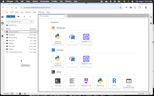
Figure 2. Screenshot of Jupyter Lab. Select R icon under Notebook to set IRkernel.
Ready to go, Figure 3.
Figure 3. Screenshot of Jupyter Notebook running the IRkernel.
Set the runtime to R (Fig 4).
Figure 4. Screenshot of Jupyter Console running R.
It’s easy to switch kernels. Let’s say you started Jupyter Lab and notice that Python is running (Fig 5). Click on the kernel name — see green arrow in Figure 5 — to bring up a popup menu, Fig 6.
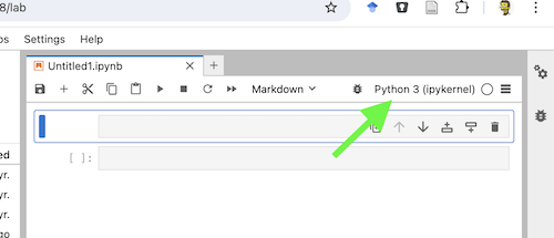
Figure 5. Screenshot of Notebook with Python set as kernel.
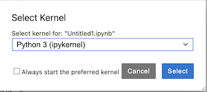
Figure 6. Screenshot of select kernel popup menu.
Click on the drop arrow and select R kernel (Fig 2), then click on blue Select button (see Figure 7).
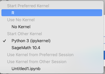
Figure 7. Screenshot of installed kernels.
Confirm R is running (Fig 8, green circle).
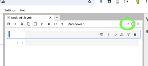
Figure 8. Screenshot Jupyter Notebook, confirm R runtime is set (green circle).
References and additional resources
Kluyver, T., Ragan-Kelley, B., Pé, Rez, F., Granger, B., Bussonnier, M., Frederic, J., Kelley, K., Hamrick, J., Grout, J., Corlay, S., Ivanov, P., Avila, D., n, Abdalla, S., Willing, C., & Team, J. D. (2016). Jupyter Notebooks – a publishing format for reproducible computational workflows. In Positioning and Power in Academic Publishing: Players, Agents and Agendas (pp. 87–90). IOS Press. https://doi.org/10.3233/978-1-61499-649-1-87
JupyterLab Developers. (Ongoing). JupyterLab Documentation. jupyterlab.readthedocs.io
Project Jupyter. (Ongoing). Project Jupyter Documentation. docs.jupyter.org
/MD
Use R in the cloud
Download pdf file of this page
Introduction
This page provides a limited guide about how to how to run R via a cloud computing (serverless) option. For local installation of R onto a personal computer, please see Install R.
My suggestion for BI-311 students — use Google CoLaboratory. However, do explore each option to find your favorite way to interact with R in the cloud. For example, the sandbox options are great for testing code snippets.
Installation guides quickly become outdated. This page last updated 12 August 2025 and describes working installation protocols at that time.
Jump to quick links for different cloud environments
- myCompiler
- JupyterLite
- CoCalc by SageMATH
- Google CoLaboratory ← Dohm’s preferred choice
- RStudio in the cloud
- rdrr.io
Example R code snippet
Below you’ll find brief introductions to five different cloud options for running R. For your convenience, the example R code I run is listed below
myX <- c(1,2,3,4)
myY <- c(5,10,15,20)
plot(myY, myX)
Bonus: Since Descartes and the Cartesian coordinate system, by convention we place the X variable on the horizontal axis. Confirm and, if necessary, alter the provided code with smallest number of changes to yield a scatter plot with X variable on horizontal axis and Y variable on vertical axis.
Run R on your computer (ie, local development environment or LDE)
This page is about running R in the cloud, a server-less options. For installing R and R Commander onto your own computer (= your LDE option), see Install R and Install R Commander.
Note 1: You cannot install R Commander to any cloud server option. R Commander requires access to a local graphical display; in the cloud, all interactions between you and R are accomplished via the web browser.
Run R “in the Cloud”
If you do not wish to install R, or, if you have a ARM-based Chromebook and, therefore cannot gracefully install R, then there are alternatives; Run R in the Cloud. I’ll list five ways to run R in the cloud — run R on a server, not your own computer — for free.
Note 2: JupyterLite, Google CoLab, CoCalc, and RStudio in the Cloud offers a free version that is generally sufficient for BI-311 coursework. However, the free service has limitations, such as reduced computing resources, session timeouts, and occasional downtime. Paid CoLab Pro options are available but not required for this course. All exercises in this Workbook are designed to run on the free version.
If you have a Chromebook, or you want to run R on your tablet (iPad, Kindle, etc.), you can’t typically install R to any of these devices (see Linux distros for limited exception for some Chromebooks). However, you can access R via a serverless Cloud solution.
Note 3: myCompiler (#1), JupyterLite (#2), and rdrr.io (#6) are examples of code playgrounds or sandboxes. These are great for running small amounts of code — like solving a homework problem. Playgrounds shouldn’t be used for larger projects and you shouldn’t expect all R packages will run in playgrounds. The other disadvantage, you probably shouldn’t mount your Google drive in a code playground!
1. Run R code at Online R Compiler using myCompiler‘s online IDE, link at https://www.mycompiler.io/online-r-compiler. Example of myCompiler and R screenshot shown in Figure 1.
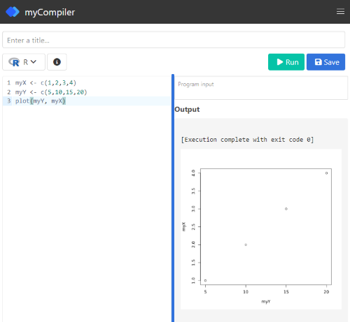
Figure 1. Screenshot of myCompiler session.
myCompiler runs dozens of programming languages. MIT’s “Try It Online,” seems to be tops at this, with access to hundreds of programming languages, including Pascal — which takes me back to my graduate student days.
2. JupyterLite uses WebAssembly to run Python code within the browser. It’s a good option to try code snippets. Like all JupyterLab options, the default environment is Python. The home screen provide options to “launch” different coding environments and R is one of the options. In general, choose the Notebook options, although note that you can load and edit markdown files. For additional information about running R code relevant to Jupyter Notebooks see step 4a or step 4b below.
3. Run code snippets in CoCalc by folks at SageMath and available at https://cocalc.com/ . CoCalc uses Jupyter Notebooks, a wonderful, open-source project which supports interactive computer coding for many languages, including R and Markdown.
While CoLab is my go to, CoCalc is a really good student option — hint: I have my Systems Biology students use this option — includes SageMATH, python, GNU Octave and other software.
Create a free account (you’ll then be able to save your code), or simply click “Run CoCalc Now” and check the box to agree to the terms to begin a session (Fig 2). Choose to open a new Jupyter notebook, then select R (system wide) from the choice of kernels.
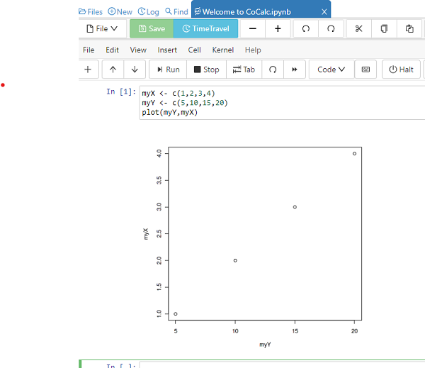
Figure 2. Screenshot of CoCalc session.
You can load files from your computer for use in CoCalc sessions. There is also a version of the software you can download to your computer.
4. My favorite option for running R in the cloud is to run R code snippets at Google Colaboratory (Fig 3). Like CoCalc, Colaboratory uses Jupyter Notebooks. One real advantage of choosing CoLab, there are apps to run Google Colaboratory and Jupyter Notebooks on iPad/iPhone and for Android phones are available at Apple App Store and Google Play, respectively.
Note 4: Google CoLab runs python by default. Because the runtime resets with each session, you’ll need to reset the runtime to R each time, following these listed steps (4a). Alternatively, leave the python environment as is an run R commands via magic commands and rpy2.ipython extension (listed below at 4b).
4a. Setup CoLab for use in the cloud is straightforward, just four steps as of August 2025.
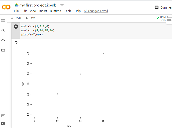
Figure 3. Screenshot of Google Colab session.
Step 1. Log in to your Google account (or create one if you don’t already have one).
Step 2. Click the url link https://colab.research.google.com/#create=true&language=r , or try the short URL https://colab.to/r. Alternatively, if you prefer, here’s a qrcode (Fig 4).

Figure 4. QR code with url to create new R notebook in CoLab.
Step 3. After creating a notebook, you’ll want to connect to your Google Drive to upload data files and script files, and to save files from R sessions.
# Install and load the functions needed to connect to Google drive
install.packages("googledrive")
library(googledrive)

# Authenticate your account
drive_auth(use_oob = TRUE)
The instructions call for you to click on web link and copy from the web page an authorization code (green arrow, Fig 5).

Figure 5. Screenshot of “Complete the Google auth process” page.
Copy the authentication code and paste it into the space provided on the colab notebook.
Step 4. You’ll want to rename and update the file name. Note in Figure 3 that the notebook name has the .ipynb file extension. Because we’re running R, don’t forget to change from the Python file extension to the .R file extension.
You’re ready to run your R code.
To confirm use of R as opposed to Python (the default language), from the menu bar select Runtime → Change runtime type and confirm R is the runtime type (Fig 6).

Figure 6. Screenshot, confirm R is the programming language in use by the Google Colab session.
After completing a session, hide code you do not want to share and print the notebook to a pdf file.
Colabs is worth the effort — you end up with a system to run R in your browser, it’s free to use, and you can store/retrieve files from your Google Drive. This is my choice for Cloud computing, and it’s the most generic solution. Starting in Fall 2025, we use Google CoLab in my biostatistics course at Chaminade University.
For more information about R and CoLab, see post by Ed Adityawarman, How to use R in Google Colab.
Colab Jupyter notebooks use Python by default. To run R, either use the link listed above each time you want to create a new R notebook, or add the following code snippet to your new notebook page
4b. Run R from within Python environment in your Jupyter Notebook by use of “magic”
# activate R magic - must begin each R code with %%R
%load_ext rpy2.ipython
For all subsequent R code, start the section with
%%R
myX <- c(1,2,3,4)
myY <- c(5,10,15,20)
plot(myY, myX)
Code and output displayed in Figure 7.
Note 5: %%R is for use with multiple lines of code. If only one line, then use %R.

Figure 7. Screenshot magic function rpy2 in action on CoLab, python environment.
Note 6: Jupyter Notebooks are a fantastic development in data science, particularly for collaboration. Although not a focus on my course, serious students may want to explore the Jupyter Notebook environment further (see Kluyver et al 2016). For example, you can install Jupyter onto your computer via Miniconda — conda is an open source package management system but then, you still would have to install R to your computer.
5. You can run RStudio at Posit Cloud. Registration and use is free for students. This works OK, but can be slow and it’s hard to work on your own data (free plan allows 25 projects and no more than 25 hours of computing time). It does have the advantage of providing the familiar RStudio interface. No doubt, RStudio is the predominate tool used by R programmers.
Choose the free plan; Instructions to get started are at https://posit.cloud/plans. You can link to your Google Drive in cloud version of RStudio via the googledrive package (introduced above with instructions for Google Colab).
A screenshot of an RStudio cloud session is shown in Figure 8.
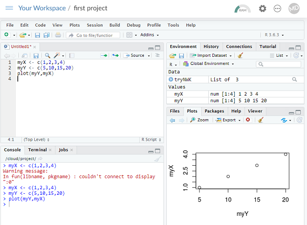
Figure 8. Screenshot of RStudio at Posit Cloud session.
6. For limited use, ie, you just need to run a little code to solve an assignment problem, you can run R code snippets in your browser at rdrr.io/snippets/ (Fig 9). You’ll see many of my code embedded in this service so that you can run code snippets from my Chaminade University CANVAS pages.
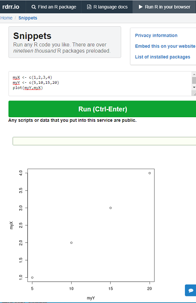
Figure 9. Screenshot of rdrr.io/snippets session.
References and additional resources
Kluyver, T., Ragan-Kelley, B., Pé, Rez, F., Granger, B., Bussonnier, M., Frederic, J., Kelley, K., Hamrick, J., Grout, J., Corlay, S., Ivanov, P., Avila, D., n, Abdalla, S., Willing, C., & Team, J. D. (2016). Jupyter Notebooks – a publishing format for reproducible computational workflows. In Positioning and Power in Academic Publishing: Players, Agents and Agendas (pp. 87–90). IOS Press. https://doi.org/10.3233/978-1-61499-649-1-87
Install R Commander
Download pdf file of this page
Introduction
For beginning (bio)statistics students who need R, I recommend use of the graphic user interface, GUI, R Commander. R Commander is an R package. It’s a large package, and requires installation of many additional packages. Generally, these additional required packages are also installed with the installation of R Commander.
This page provides a guide about how to install R Commander onto your computer (LDE). To use R Commander, please see Chapter 1.1 – A quick look at R and R Commander. You must have R installed and working correctly on your computer before proceeding to install the R Commander package. Click here to get the Install R guide.
Note 1: If you plan to run R in the Cloud, you cannot install the R Commander package, which must be part of a local development environment.
Installation guides quickly become outdated. This page last updated 12 August 2025 and describes working installation protocols at that time. Like all secondary guides to software installation, I recommend reading installation notes by the coders who provide the software. For R Commander, see R Commander Installation Notes, by Dr John Fox.
For your convenience, the example R code I run is listed below
myX <- c(1,2,3,4)
myY <- c(5,10,15,20)
plot(myY, myX)
For BI311, we also use R Commander
R Commander is a package that adds function to R; it provides a familiar point-and-click interface to R, which allows the user to access functions via a drop-down menu system (Fox 2017). Thus, instead of writing code to run a statistical test, Rcmdr provides a simple menu driven approach to help students select and apply the correct statistical test. R Commander also provides access to Rmarkdown and a menu approach to rendering reports.
RStudio is another way to interact with R, and compared to R Commander, is designed to help R programmers with a useful environment to manage files, generate reports, and work on R code. I continue to use R Commander in teaching because it emphasizes statistics and note coding. One advantage of R Commander for learning how to code with R is that code is reproduced from student’s selections in the drop-down menu options.
Note 2: A couple of years ago the folks at Posit, who publish RStudio, introduced the IDE Positron. I won’t comment about this IDE, but point interested readers to a page at R-Bloggers: Positron vs RStudio – is it time to switch?
Install R Commander
To install R Commander, enter the following code at the R prompt. See Figure 1 below for a screenshot of the R Commander interface.
install.packages("Rcmdr")
In addition, download and install the plugin
install.packages("RcmdrMisc")
Note: You can combine requests as follows
install.packages("Rcmdr", "RcmdrMisc", dependencies=TRUE)
Adding “dependencies=TRUE” will also install other packages that Rcmdr needs (which would get downloaded once you start Rcmdr for the first time).
If you have not set a mirror site, you’ll be prompted to do so before you can download and install packages. I recommend 0-Cloud as default mirror site. Be advised: because our university shares a single public IP address, you may experience download delays if we all try to use the same mirror site at the same time.
To start R Commander, load the packages via the library() command.
library(Rcmdr)
Follow installation prompts. You can skip adding the “otools,” for now. However, Rcmdr will prompt you to install otools every time you start, so go ahead and install them at your convenience.
MacOS users: To improve Rcmdr performance you must turn off “app nap.” From Rcmdr, go to Tools, then select “Manage Mac OS X app nap for R.app …” Once you select “off” (click OK to apply), restart Rcmdr, the delay will be removed. Windows 11 folks don’t have to contend with nap.
Test Rcmdr
Figure 1 shows a basic R Commander session. Enter code in the script window (1), click on the Submit button to run the code, and results show up in the output window (2). Figure 1 shows R Commander opened in a MDI.
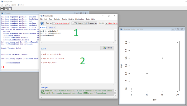
Figure 1. Screenshot of basic R Commander session on WinPC.
Click on R Markdown tab, edit (e.g., replace with your own title and name), then click on the Generate Report button to create a pdf of your work, default file name is RcmdrMarkdown.pdf (Fig 2). If you do not have pandoc and LaTeX properly installed, then only an HTML document will be available as an option.
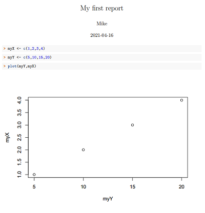
Figure 2. Screenshot of portion of RcmdrMarkdown.pdf.
Although I don’t recommend this practice, you can run R Commander from within RStudio. The downside is that multiple windows may be generated (Fig 3), which can be challenging for new users to navigate. On Windows pc some of this behavior can be controlled by selecting the SDI windowing option as opposed to the default MDI windowing option.

Figure 3. Screenshot of basic R Commander session in RStudio on macOS.
Note 5: Recent versions of macOS offer “Stage Manager” and “Split View” options which can help manage a project that requires two or more apps open and available for use. On Windows PCs, Snap Layouts allow up to four apps to be quickly arranged for easy access.
Add pandoc and LaTex support
To complete your R Commander installation you may want to add additional document handling software, LaTex and pandoc. R Commander already contains R Markdown, but these additional software allow you to take advantage of “high-quality typesetting.”
Note 6: BI-311 students: It’s not necessary to install pandoc and LaTeX. With the included RMarkdown options in R Commander, the default page generated is an html (web) document, which will be displayed in the default browser. BI-311 reports are submitted as pdf files — therefore, it’s a straightforward to save the html page as a pdf within the browser. For example, Google Chrome select Print, then select save as pdf for the destination.
In Rcmdr, select Tools from the menu, then Install Auxillary Software. Click OK, which will open links in your default browser to download pages for LaTex and pandoc. Download the files, follow the installation instructions for pandoc and LaTeX, then restart R and Rcmdr.
Here are direct links to the files, plus installation notes
LaTeX — links verified 27 August 2025
MikTeX from https://miktex.org/download:
- for Windows systems, select
basic-miktex-24.1-x64.exe - for MacOS, select
miktex-22.1-darwin-x86_64.dmg
pandoc — links verified 12 August 2025
Windows 11
https://github.com/jgm/pandoc/releases/download/3.7.0.2/pandoc-3.7.0.2-windows-x86_64.msi
MacOS
ARM CPU (M1 – M4): https://github.com/jgm/pandoc/releases/download/3.7.0.2/pandoc-3.7.0.2-1-arm64.deb
INTEL CPU: https://github.com/jgm/pandoc/releases/download/3.7.0.2/pandoc-3.7.0.2-x86_64-macOS.pkg
/MD
Install R
This page has 30 images
Introduction
The first time installing R can seem intimidating. To start, be clear about the overall goal of the procedure: providing the student with an accessible environment for solving statistics problems.
In brief, this page explains how to get R set up on your computer. First, you need to download the R installer from the official CRAN website. When you run the installer,in general, accept the default choices. However, for Windows users, it’s important to right-click the file and choose “Run as administrator.” This step ensures that R has the proper permissions to install correctly and avoids problems with user access later on. Once installed, you can open R and test it by typing a simple command like `2 + 2` in the console to confirm everything is working.
The flow chart presented in Fig 1 suggests a way to orient the student to solving the task. First, understand which type of computing environment you have available. Second, if a macOS, then additional software (XQuartz) is required to provide full function to the R software. Third, download and install the base R software appropriate for the computer system.
Figure 1 suggests an R installation flow chart.
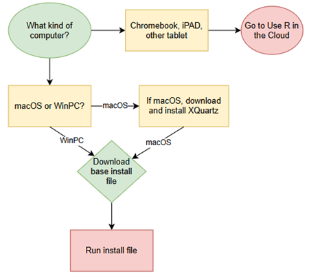
Figure 1. Suggested flow chart for R installation.
Note 1: I skipped Linux in the flow chart — I’m working on the assumption that Linux users are more comfortable installing 3rd party software. However, some notes on R installs on Linux distros are included on this page.
It’s possible to follow the steps in Figure 1, accepting all default options presented along the way, to end up with a working R environment. As with many software processes, there are choices beyond defaults that can be made to improve the software use.
This page presents a detailed guide about how to install R onto your computer — this is referred to as building a local development environment or LDE. Additional install R help was provided in Chapter 1.1 – A quick look at R and R Commander.
Instructions for RStudio are also provided (optional for BI311 students). A guide to install R Commander is provided in Install R Commander.
Instructions for how to run R via a “cloud computing” (serverless) option — a remote development environment — are also provided, Use R in the Cloud.
For help upgrading installed packages after upgrading new R version, see R packages.
Note 2: Installation guides quickly become outdated. This page was created first in September 2019 and last updated August 2025 and describes working installation protocols at that time. As of August 2025, R -4.5.1 was current version. Instructions for Win10 and Win11 are the same. Instructions for Intel-based macOS are the same; with Apple’s switch to ARM64 (M1, M2, M3, M4), changes have been made. Going forward, the instructions on this page, but not my videos — version numbers need to be updated in the videos, are likely to be the same for new R versions. And wow! Search Google or Bing for “how to install R,” options in the millions. Ultimately the best source is in the R installation and administration manual.
Per usual caveat about this page of instructions: my advice is offered for instructional purposes and in no way implies warranty against damage or guarantee of success.
Run R on your computer (LDE install)
CoLab, skip this step: Instead, go to Use R in the cloud.
So why in this day in age should you install and build R on your own computer? The remote options to run R in the cloud are a wonderful option, convenient: you can access anywhere you have internet, from any device that connects to the internet. It’s easy to share and work together on projects, particularly those based on Jupyter Notebooks.
I think the main benefits to a local installation is it’s a more efficient environment to work in — you have control of everything and, provided your PC has power, a working R install on your computer will always be available to you. Since you can control the update cycle for your computer, you won’t run into times you cannot access the remote server to work on your project. Testing code is faster on a local install, feedback — think error messages — apply to your installed version. And, while remote R servers may come with low initial costs to students, any significant use will quickly require paid accounts. As a reminder, the good folks at the R-project continue to offer R as free software. All you need to do is work through the install process.
Start at the R-project homepage, r-project.org. To download software, first click on CRAN link, located on left hand side of the screen (here, highlighted by green arrow, Fig 2).
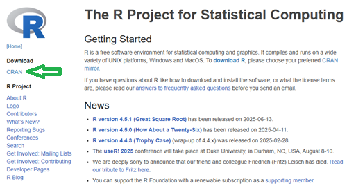
Figure 2. Screenshot homepage for R-project.org.
Figure 3 shows a screenshot of the CRAN mirror page. The idea is to select the mirror site closest to your location. In Hawaiʻi, that’s likely to be any of the sites in California. However, I recommend selecting the first in the list, 0-cloud, at cloud.r-project.org (highlighted by green arrow, Fig 3).
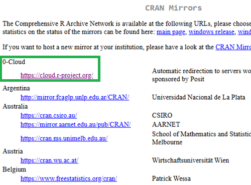
Figure 3. Screenshot of portion of R-Project CRAN mirror page.
Note 3: After installing R, see this page to learn how to set the CRAN mirror.
After selecting the mirror site, the download page is presented (Fig 4). Click on the link that corresponds to your computer system (Linux, macOS, or Windows).
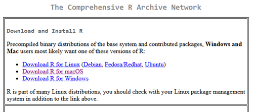
Figure 4. Screenshot of portion of base R download page.
Once the installation file is located onto your computer, proceed to install base R.
Detailed instructions
For screenshots of installation steps on WinPC, see Win10/11 setup, screenshots
- Windows PCs, download the base application from selected CRAN Mirror site, select Download R for Windows, and install the R software as you would any other software. All of you are likely to have the 64-bit version of Windows 11, so install the 64-bit version of R. Follow the instructions as they are presented. Screenshots of the install process are available at the end of this page (click here or scroll down to Win11 setup, Screenshots).
- Current versions of Microsoft Windows come in several flavors, the simplest distinction is between home and pro. R runs perfectly well on both.
- Windows 10 is reaching end of life cycle.
- Some inexpensive Microsoft Windows PCs are built on ARM64, not Intel or AMD64 CPU. Thus, installing R and or RStudio may prove problematic.
- Also note: Windows in S mode only run applications from the Microsoft store. To install R, you first may need to switch out of S mode (see Microsoft FAQ about S mode).
- You should install R with Administrator privileges. Highlight the install file, right-click the file, and select “Run as administrator” from the popup menu.
- When you first try to run R you may get a popup screen “Windows protected your PC,” locate and click on the “More info” link and select “Run anyway.”
- This in no way will harm your computer — provided you have downloaded from official sites. R is a verified program. Microsoft has taken an aggressive line on developers and favors apps that are part of their app store.
- It is advisable to confirm for yourself: check the md5sum against the fingerprint on the CRAN server
- When prompted, I recommend that you change the install directory to root folder, e.g.,
C:\R\R-4.5.1. This will allow for installation of packages to the common library as opposed to a personal library.- I recommend this change because of how Windows assigns home folders. During initial setup Windows 10 prompted you to choose a username and whether you wanted your work stored locally or in your OneDrive folder. A worse case scenario? You select a username with spaces, e.g.,”Mike Dohm,” and you selected OneDrive. Both will cause challenges later for running and or installing packages for R.
- If you install R anywhere but the default Program files folder on your Win10/11 PC, chances are you will need to add the folder containing the executable, r.exe, to you path.
- Search: “env”
- Open “Edit the system environment variables” in the Control Panel
- Click Advanced tab, then click on Environment Variables… button (lower right of panel)
- Under System variables, scroll to and select Path.
- Click Edit… button, then click New button.
- Type in the path to the folder containing R.exe. That’s likely to be C:\R\R-4.5.1, assuming R-4.5.1 is the latest version of R installed on your computer.
- If you install R anywhere but the default Program files folder on your Win10/11 PC, chances are you will need to add the folder containing the executable, r.exe, to you path.
- I made a video for you. Video is about 26 minutes long; at 22 minute mark, video includes how to install R Commander (instructions provided Install R Commander).
- Apologies for the production quality — videos are not my thing.
- I recommend this change because of how Windows assigns home folders. During initial setup Windows 10 prompted you to choose a username and whether you wanted your work stored locally or in your OneDrive folder. A worse case scenario? You select a username with spaces, e.g.,”Mike Dohm,” and you selected OneDrive. Both will cause challenges later for running and or installing packages for R.
- Current versions of Microsoft Windows come in several flavors, the simplest distinction is between home and pro. R runs perfectly well on both.
For screenshots of installation steps on WinPC, see MacOS setup, screenshots
- macOS PCs, first you must download and install XQuartz from https://www.xquartz.org. Best to restart your mac after installing XQuartz then proceed to install R.
After installing XQuartz, then return to https://cran.r-project.org, select Download for Mac(OS) X, and run the installer. Screenshots of the install process are available at the end of this page (click here or scroll down to Macos setup, Screenshots).- As of August 2025, be advised that there are two distinct R versions for your MacBook or iMac.
- For MacBook or iMac with Apple’s M1 or M2 ARM chip sets, download and install
R-4.5.1-arm64.pkg.- If you recently purchased a new MacBook or iMac (2020 to present), then you probably have the M2 or M3 chipset (check by clicking the Apple icon, then selecting About this Mac or System Information (
/Applications/Utilities/System Information.app)). - XQuartz version 2.8.5 works on macs with either the M1 or Intel chipsets.
- If you recently purchased a new MacBook or iMac (2020 to present), then you probably have the M2 or M3 chipset (check by clicking the Apple icon, then selecting About this Mac or System Information (
- For older MacBook or iMacs with Intel processors, download
R-4.5.1-x86_64.pkg. Depreciated 8/4/2021: Be advised that these instructions are for Intel-based macs. At the time of writing these instructions (April 2021), the installation of XQuartz and R should work on new M1-based macs. At the time of this writing (April 2021), however, R will not run natively on your M1 mac. It will run using Rosetta 2, an emulator that is included with your M1 mac. The R folks are busy working on a version that will run natively, which may be ready within a few months.
- For MacBook or iMac with Apple’s M1 or M2 ARM chip sets, download and install
- At the completion of the install process, don’t forget to drag the R app to your Applications folder.
- When you first try to run R, you may get a popup screen which provides no option to start the app, and perhaps even a rather ominous option to move the app to Trash. Just close the warning message and right-click on the R app. A new screen pops up, which looks very much like the previous warning, but now you will see and option to open the app. Click on open to start R.
- Like the message to Windows PC users, bypassing Apple’s Gatekeeper to run R in no way will harm your computer — provided you have downloaded from official sites — R is a verified program. Apple has taken an aggressive line on developers and favors apps that are part of their app store.
- As of August 2025, be advised that there are two distinct R versions for your MacBook or iMac.
- LINUX distros. If your PC platform is Linux, then you should be comfortable with installation and updating of software. R base is already included in Debian distributions (e.g., Mint, Ubuntu). See https://cloud.r-project.org/ for additional instructions.
- For Chromebook users, if you can install a Linux subsystem, then you can also install and run R. For instructions to install R see Levi’s excellent writeup at levente.littvay.hu/chromebook/.
Note 4: To install up-to-date R and RStudio, your Chromebook needs to have Intel or AMD CPU; my ASUS Chromebook has an ARM64 processor (MediaTek mt8183), and Levi’s instructions don’t apply. As of January 2024 I am pushing the installation process a bit on my little Chromebook and have successfully created the Linux container (Debian 11, Bullseye) and installed base (and development) R version (4.0.4) included with the Linux distribution. Stay tuned — I’ll update progress with installing an R environment on ARM64-based Chromebook.
Update August 2025 — no change, very challenging to get R environment running and updated on ARM64 Chromebook. RStudio not possible.
Test R
For both macOS and Windows PCs, successful installation of R on your computer installs base R programming language and a simple graphical user interface. Test your install by running code in the terminal (one line at a time) or via script:
- Rgui.exe (Windows PC)
- File → New script
Enter code in script editor, e.g.,
myX <- c(1,2,3,4)
myY <- c(5,10,15,20)
plot(myY,myX)
- Run code: Ctrl+R
Figure 5 shows screenshot of R running on WinPC. RGui.exe (1), script editor (2), and results of plot() (3) on WinPC.
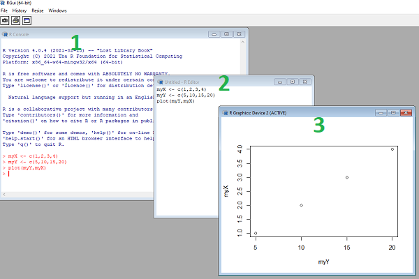
Figure 5. Screenshot of RGui.exe (1), script editor (2), and results of plot() (3) on WinPC.
- R.app (macOS): run code in the terminal or via script
- File → New Document
Enter code in script editor, e.g.,
myX <- c(1,2,3,4)
myY <- c(5,10,15,20)
plot(myY,myX)
- Run code: Cmd+Enter
Figure 6 shows screenshot of R running on macOS. R.app (1), script editor (2), and results of plot() (3).
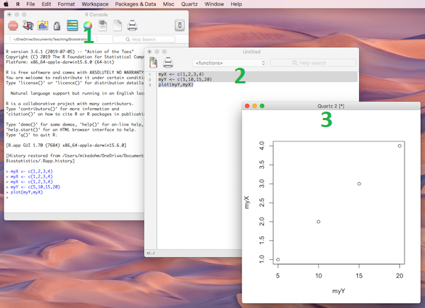
Figure 6. Screenshot of R.app (1), script editor (2), and results of plot() (3) on macOS.
Many of you would like a video. Do a little search and you’ll find plenty, although most are also showing how to install RStudio in addition to base R.
Note 5: For my Biostatistics class, BI311, we typically will run R and use R Commander for scripting, without RStudio.
For BI311, we also use R Commander package
R Commander is a package that adds function to R; it provides a familiar point-and-click interface to R, which allows the user to access functions via a drop-down menu system (Fox 2017).
Go to Install R Commander guide.
Personalize R startup
To add function to R, you’ll download many R packages. These, too, are stored at the mirror sites. Each time you run install.packages(), R will ask for the mirror site. The R app on Windows pops up a long selection box; macOS R.app is a bit more friendly, but regardless, it’s best to choose a mirror site at the beginning of a session. At the R prompt, type and submit the command
options(repos = c(CRAN = "https://cloud.r-project.org"))
this will remain in effect for the current R session.
To make the change permanent, add to .Rprofile — a hidden file — in your personal home directory
local({
r <- getOption("repos")
r["CRAN"] <- "https://cloud.r-project.org"
options(repos = r)
})
If you use textedit or notepad, make sure to return after the }); the file requires an empty new line to run.
Restart R, then enter at the prompt
file.exists("~/.Rprofile")
If you’ve created the Rprofile file correctly, R should repeat.
Run R from the terminal
Whether yours is a mac or win11 pc, you have a powerful computing environment lurking beneath the glossy graphic user interface. It’s called the terminal. The terminal is a place where text-based instructions may be written and submitted to command your computer to do something.
On win11 pc, the modern terminal is the Power Shell. Search “PowerShell,” then open Windows PowerShell. Alternatively, shortcut + X, then I key. This opens terminal in your home folder.
- You’ll want to navigate to your working folder, e.g., BI311 on the Desktop. Setting your working folder can be done in R of course, but at the terminal type the command “
cd \users\default\desktop\bi311“.
On macOS, Spotlight (search) “Terminal.app“. Alternatively, right-click on your working folder icon and select New terminal at Folder from the popup menu.
On Ubuntu Linux, shortcut keys + alt, then t key.
Open the included script editor
Use RStudio
Rstudio is a very popular data science IDE, specifically written for R programming. Therefore, if your goal is to become adept at R programming, go with RStudio. Like R Commander, Rstudio provides an environment to write an manage code, generate markdown reports, and importantly, manage files in R projects. Figure 7 shows a screenshot of RStudio: Clockwise, four panes: Source, Environment, Output, Console on WinPC. BI311 students, please note that I recommend use of R Commander and Google CoLab.
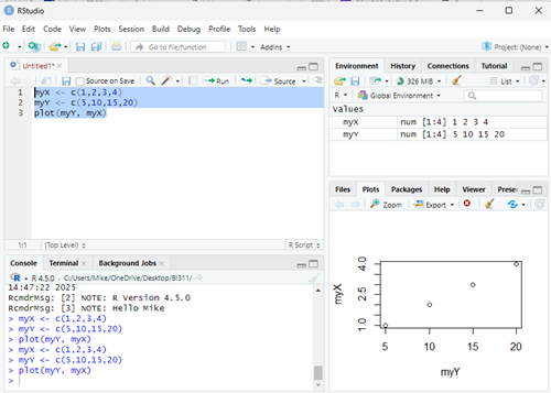
Figure 7. Screenshot of RStudio IDE.
Installation of RStudio desktop is straightforward.
Go to https://posit.co/download/rstudio-desktop/
Install R first. Since at this point you’ve likely already installed R, go directly to 2 (green box, Fig 8).
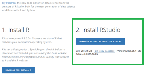
Figure 8. Screenshot RStudio desktop download page, current as of September 2025.
After downloading the installation software, double click the file to begin. Follow on screen instructions for your computer system.
Run R in the “Cloud”
If you do not wish to install R, or, if you have a Chromebook and, therefore cannot gracefully install R, then there are alternatives; Run R in the Cloud. I’ll list three ways to run R in the cloud for free. Go to Use R in the Cloud guide.
MacOS setup, Screenshots
Download R install package from R-project.org, then select the R install package from your Download folder (Fig 9).
Note 6: The following screenshots were for previous R version 4.1.1. As of Fall 2025, current R version is 4.5.1. The screenshots are consistent between the current and older versions of R on macOS.
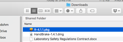
Figure 9. Screenshot — Find the R install file in your download folder.
First screen, R install for macOS (Fig 10). Select continue.
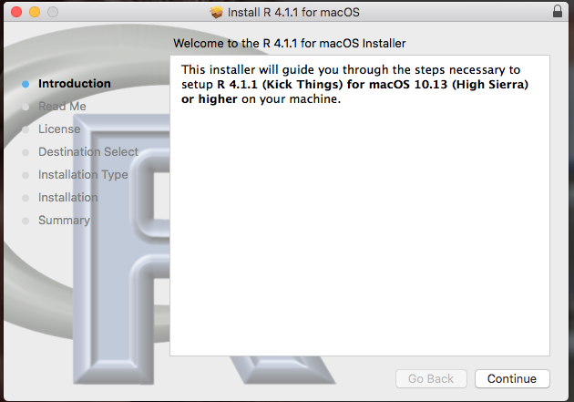
Figure 10. Screenshot: first instructions pop-up window.
Second screen, R install on macOS (Fig 11). Select continue.
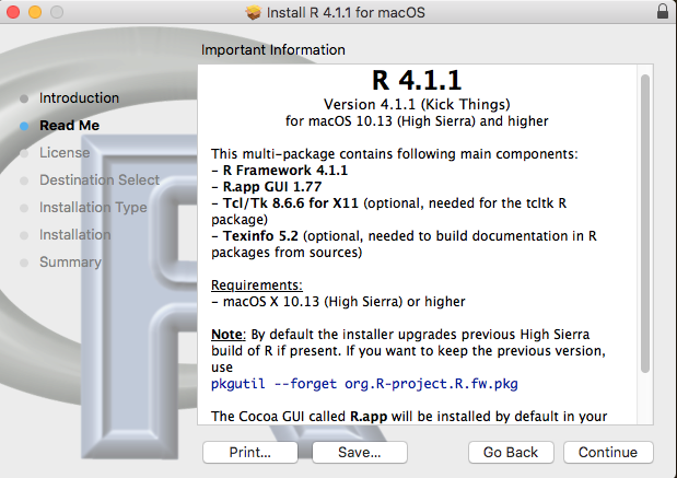
Figure 11. Screenshot: second instructions pop-up window.
Third screen, R install on macOS (Fig 12). Select continue.
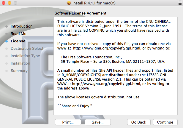
Figure 12. Screenshot: third instructions pop-up window.
Fourth screen, R install on macOS (Fig 13). Agree to continue.
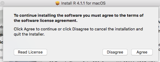
Figure 13. Screenshot: fourth instructions pop-up window.
Fifth screen, R install on macOS (Fig 14). Select Install.
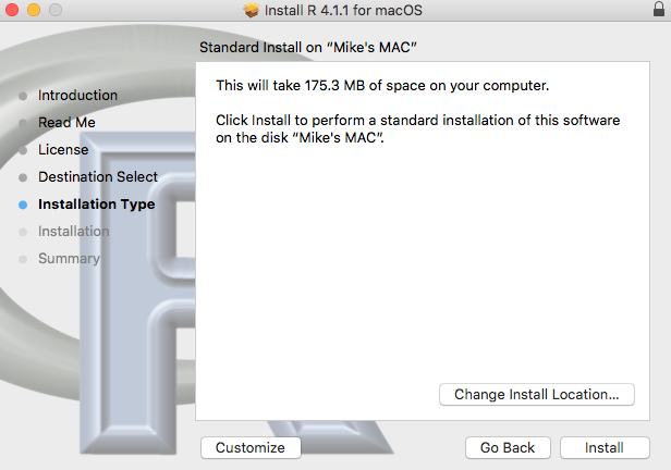
Figure 14. Screenshot: fifth instructions pop-up window.
Sixth screen, R install on macOS (Fig 15). Enter your username and password for your computer, then select Install Software.
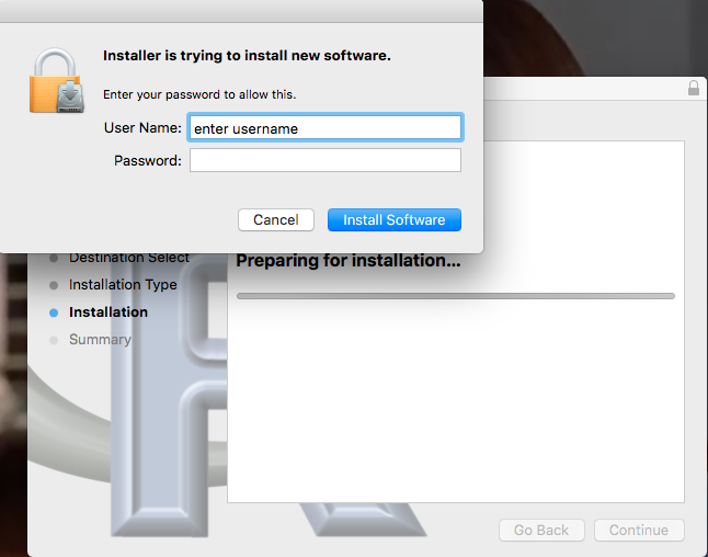
Figure 15. Screenshot: sixth instructions pop-up window.
Seventh screen, R install on macOS (Fig 16). Several screens will popup, reporting progress. Be patient!
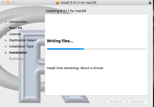
Figure 16. Screenshot: seventh instructions pop-up window.
Eighth and final screen, R install on macOS (Fig 17). Select close.
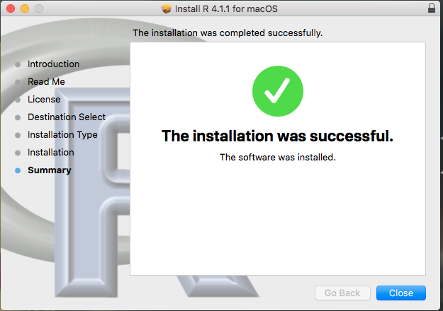
Figure 17. Screenshot: eighth and final instructions pop-up window.
Optional — Keep or discard the install file (Fig 18). I keep and then do manual delete after I’ve confirmed the installation.
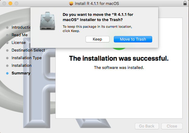
Figure 18. Screenshot: MacOS will prompt with option to delete the installation file. This has no effect on the installation of R.
From Applications folder, start R.app. You should see the R Console (Fig 19).
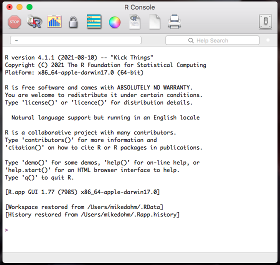
Figure 19. Screenshot: R Console in the R.app on macOS.
Wind10/11 setup, screenshots
Download from R-project.org, then right-click the R install package from your Download folder. Run as administrator (Fig 20).
Note 7: The following screenshots were for previous versions of R, 3.6.1 and 4.0.5. As of Fall 2025, current R version is 4.5.1. The screenshots are consistent between the current and older versions of R on Windows 10/11.
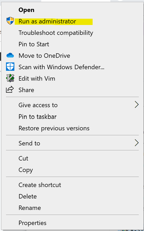
Figure 20. WinPC screenshot: Pop-up menu after right-click on the R installation file in windows Explorer.
First screen, select language (Fig 21). Select OK to continue
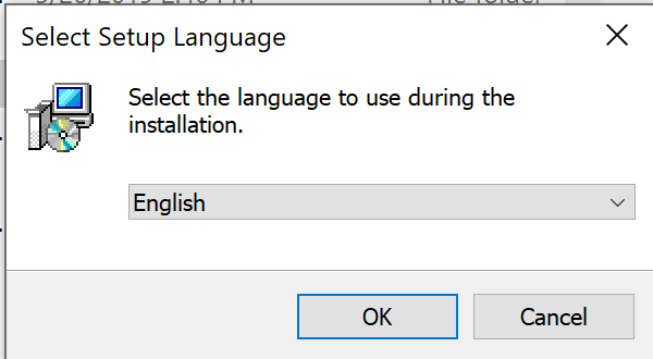
Figure 21. WinPC screenshot: first instructions pop-up window.
Second screen (Fig 22), click Next to continue
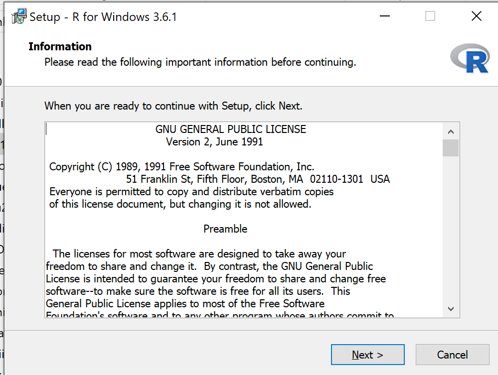
Figure 22. WinPC screenshot: second instructions pop-up window.
Third screen (Fig 23). Change the default location (show in the screenshot) to root folder, e.g., C:\R\R-4.5.1 (current version as of August 2025).
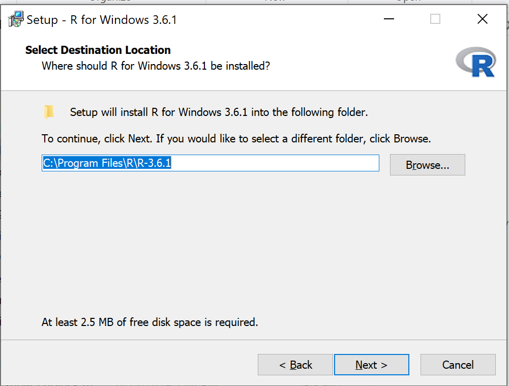
Figure 23. WinPC screenshot: third instructions pop-up window. Note — R-4.5.1 (current version as of August 2025).
Fourth screen (Fig 24). Change startup options. Select Yes (customized startup) to continue.
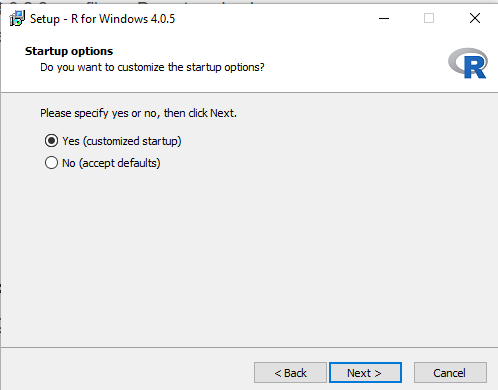
Figure 24. WinPC screenshot: fourth instructions pop-up window.
Fifth screen (Fig 25), select SDI — single document interface — not the default MDI — multiple document interface, then Next to continue.
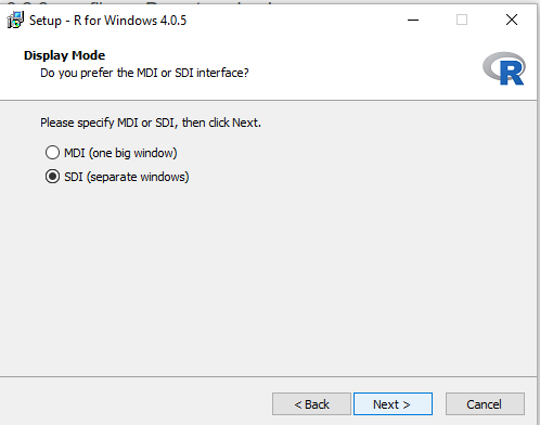
Figure 25. WinPC screenshot: fifth instructions pop-up window. Recommend setting to SDI.
Sixth screen (Fig 26), select HTML help, then Next to continue.
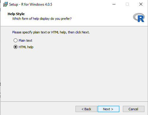
Figure 26. WinPC screenshot: sixth instructions pop-up window.
Seventh screen (Fig 27), leave start menu folder as is (R), then Next to continue.
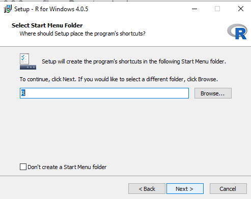
Figure 27. WinPC screenshot: seventh instructions pop-up window.
Eighth screen (Fig 28), check all boxes, then Next to continue.
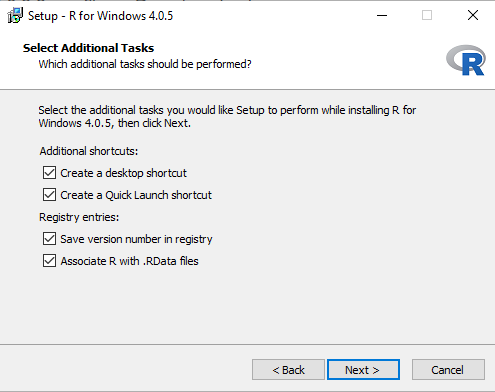
Figure 28. WinPC screenshot: eighth instructions pop-up window.
Ninth screen (Fig 29), a series of status updates during the installation.
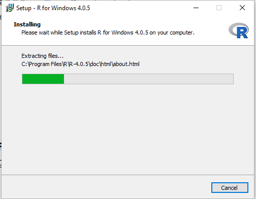
Figure 29. WinPC screenshot: ninth instructions pop-up window.
Final screen (Fig 30), successful install.
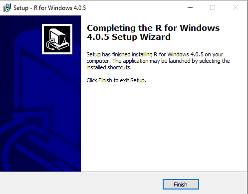
Figure 30. WinPC screenshot: final instructions pop-up window — successful installation.
/MD
2.2 – Why do we use R Software?
- Why R? The case for using R in biostatistics education.
- How to get started with R .
- Why R Commander, why not RStudio? .
- Wait! Why don’t we use Microsoft Excel? .
- Statistics comparisons between R and MS Excel .
- Graphics comparison between R and MS Excel .
- So, you’re telling me I don’t need a spreadsheet application? .
- Still not convinced? .
- Why install R on your computer?.
- Help with R?.
- Questions .
- Quiz .
- Chapter 2 contents.
If this page is TL;DR, and you’re in a rush, then instructions to install R onto your macOS or Windows PC are provided in Install R. To run in the cloud only, see Use R in the cloud.
Why R? The case for using R in biostatistics education.
.
Why do we use R Software? Or put another way: DrD, Why are you making me use R?
Truth? You can use just about any acceptable statistical application to get the work done and achieve the learning objectives we have for beginning biostatistics. However, we will use the R statistical language as our primary statistical software in this course. Part of the justification is that all statistical software applications come with a learning curve, so you’d start at zero regardless of which application I used for the course.
In selecting software for statistics I have several criteria. The software should be:
- if not exactly easy, the software should have a reasonable learning curve
- widely accessible and compatible with
allmost personal computers - well-respected and widely used by professionals
- free software
- open source
- well-supported for the purposes of data analysis and data processing
- really good for making graphics, from the basics to advanced
- capable to handle diverse kinds of statistical tests
R meets all of these criteria. R history began back in 1993 and has always been available as free software under the terms of the Free Software Foundation’s GNU General Public License in source code form. R compiles and runs on a wide variety of UNIX platforms and similar systems, including GNU/LINUX, FreeBSD, and various Linux distros like the popular Ubuntu®, in addition to their more famous Microsoft Windows® and Apple macOS® distributions. To facilitate access to the software, numerous mirror sites are available from sites around the world, with cloud.r-project.org supported by RStudio perhaps the most widely used. From January 2024 to December 2024, more than 8.5 million downloads of base R were made from the RStudio CRAN mirror site (CRAN stands for Comprehensive R Archive Network.
changelog file, which allow one to track numbers of downloads for any package from their mirror site — https://cloud.r-project.org/. Here’s the code and recent counts for downloads of R itself over a four week period .
install.packages("cranlogs")
library(cranlogs)
# How many downloads of base R around start of Fall semester?
 out <- cran_downloads("R", from = "2025-08-01", to = "2025-08-31")
sum(out$count)
R output
[1] 582524
An iterative function returning number of downloads over multiple years is provided at Part05 of Mike’s Workbook for Biostatistics.
R is straightforward to use once you learn how to work with the language, but has a steep learning curve; after all, it’s a programming language. I recommend installing the program onto your computer, but ready to go R is also available at multiple cloud services, including Google CoLab and Posit Cloud. The remainder of this page is directed at users who choose to install R to their computer, although much of the discussion holds regardless of the R environment choice, local or Cloud.
For local installs of R, I also recommend use of the GUI R Commander. Use of R Commander helps with the learning curve, and eventually, your use of code will become second nature. We don’t use RStudio, but as your skills improve, I recommend transitioning to the IDE RStudio; after the initial growing pains are behind you, RStudio likely will be a better solution over R Commander.
This discussion implies learning R programming. However, while we need statistical software to do statistics, students in my BI311 course must keep in mind that learning objectives for a biostatistics course is about the concepts and interpretation of statistics, not just use of the software. In other words, learning how to use R is not the focus of BI311 nor will you likely achieve R programming competency by the end of the semester. I certainly encourage students to strive for competency and I give frequent bonus opportunities to demonstrate coding skills during the semester.
Why R and not some other statistics software?
Thus, you might ask if the purpose of the course isn’t to learn R, why work with R instead of a more familiar app or software, eg, Microsoft Excel® (hereafter simply referred to as Excel), or Google Sheets, or even my favorite open-source office alternative, LibreOffice Calc? Or, perhaps even just one of the many online calculators, if the course learning objective is to “just” learn about statistics?
First, I believe that real data derived from real biology or biomedical problems are essential elements to a first course in biostatistics. That’s not a particularly unique perspective although I don’t have survey results of other statistics instructors to back up the claim. Real problems involve observations on multiple subjects, many variables — large data sets; this alone precludes use of hand calculations and calculators. As a corollary, we will not spend a great deal of time learning the in’s and out’s of the algorithms that form particular statistical tests. Now, do understand that there is a tremendous benefit to understanding statistics by working through the equations, by looking at the algorithms, and there’s no escaping the need for understanding that probability provides the foundation of statistics inference (Chapter 8). Thus, for most of us, the statistical software available to us provides an appropriate framework for applying correct statistical tests to our projects. Therefore, the decision is about which statistical package we should use.
Second, R is perhaps the choice in academia for statistical software. A PUBMED search found more than 1500 citations of R. Visit Robert A. Muenchen’s web page (The popularity of data analysis software, r4stats.com) to see updated statistics on statistical software use. Those of you continuing on to graduate school or to professional schools will find that many of your statistically literate colleagues use R and not one of the commercial programs. While there are many excellent commercial packages (Table 1), and in some cases you can make spreadsheet programs do statistics (typically add-ins are required), all statistical software come with steep learning curves. Thus, part of my selling point to you is that learning to use R is at the cutting-edge in your field and, given that all of the software you could use can have have their challenges, it is best to work with something that will be around and is in wide use, without the burden of a financial investment.
Table 1. A selective list of statistical software.
| Software | Student license? | Limited or full function version | macOS | Windows 11 | Fee* | Academic license type |
|---|---|---|---|---|---|---|
| GraphPad Prism | Subscription, $142 per year | Full | Yes | Yes | $202 | annual subscription |
| JMP | Yes, but with purchase of selected textbook | Limited | Yes | Yes | $100 | monthly subscription |
| Minitab | Subscription, $54.99 per year | Full | Yes | Yes | $1610 | annual subscription |
| IBM SPSS | Rental, $76 per year | Full | Yes | Yes | $260 | annual rental |
| SigmaSTAT | No | NA | No | Yes | $299 | perpetual |
| MySTAT | Yes, free | Limited | No | Yes | NA | |
| SYSTAT | No | NA | No | Yes | $739 | perpetual |
| Stata | Subscription, $94 per year | Full | Yes | Yes | $325 | annual subscription |
see Wikipedia for list of additional software
Third, what about online sites like plot.ly where, for free, you can plot and, in some cases, calculate statistics? What about the web application at Brightstat, which claims to provide an SPSS-like experience online (Stricker 2008)? While it is true that there are many wonderful websites that can perform many of the statistical tests we will use this semester, these sites are not suitable for more than occasional use.
How to get started with R.
.
A few words about my approach to the software in my biostatistics course. I note to students during the semester that our course is not a programming course, but rather, programming skills are acquired along the way. Our focus is how to do statistical analysis, how to design experiments, etc. Coding skills without understanding of the why we’re doing it is not unlike learning to cook by following a great recipe as opposed to learning about the art and science of flavor (NPR Science Friday, March 15, 2024) — the homework is solved but the why we can support our conclusions may be obscure.
We set aside the first couple of class meetings simply to setup student’s Windows PC or Apple macOS computers to do data science; for students with access to Chromebooks or iPad tablets, we need to set them up to run R in the Cloud (eg., Google Colaboratory) — in other words, there’s a lot of pre-work that can present barriers to actual doing statistics in R (or other software). Once we have the environment set up for the students, we utilize a “tell-show-do” approach to learning how to code. The “tell” part includes sharing script; the “do” part is mostly done by students outside of class as part of completing homework.
First work with the language can be frustrating, so I also encourage a “five minute” rule — if it ain’t working, stop. So, by all means when Run through a troubleshooting checklist, but please don’t continue to struggle — the gap is between the instructions and where the student is with the material — it’s a me-as-instructor problem, not a student must work harder problem!
All statistics work follows a similar workflow.
The basic workflow for a data project, using R as the primary statistical programming tool, looks like that illustrated in Figure 1.

Figure 1. A basic workflow with R.
The workflow begins with the assumption that a data set already exists. Getting the data into an R session depends on the source of the data, for example stored in spreadsheet file or from a table on a webpage. Data cleaning and processing of the data may be in order — for small and modest-sized data sets, my own preference is to do most of the data cleaning in my spreadsheet app, but R has full capabilities to handle or “wrangle” data. Next, the raw data should be stored in R session in a data frame object. Once the data frame object is available, exploratory data analysis, including summary statistics and data visualization can proceed. Higher order analytics, including statistical inference and modeling, can then begin.
The R statistical language, accompanied by additional packages to extend its capabilities beyond basic math and statistical functions, provided a complete statistical environment. R is best viewed as a programming language for statistics (data analysis), and data processing. Power users of R learn how to write scripts that do t-tests, ANOVA, regression, etc. The scripts are just lines of code that R understands and it provides the user tremendous control over analysis and inference of data sets. Because of this flexibility and power, however, R can be intimidating at first. So, we’ll start slowly with scripts, introducing just what we need to get started and build from there. We’ll be addressing R issues in more depth over the next several weeks, but for the first week, our goal(s) should be to make sure each of you knows how to start/exit R, how to create and utilize a working directory, and how to use R as a calculator. You obtain your copy of R from the R Project for Statistical Computing, available at https://www.r-project.org. Instructions to install R are provided in Install R. A ten-part tutorial to get started using R is provided in Mike’s Workbook for Biostatistics.
Note 2. A working directory or working folder is something you create on your computer to contain the files and sub-directories of a project. It sets the default location for files you may need to have R read. For example, all of your work for a course (data files, script files, Markdown files), may be stored in a folder called BI311 on your Desktop. For example, on a macOS, the path to the working folder would be
/Users/username/Desktop/BI311
Why R Commander, why not RStudio?
.
We utilize an R package that provides a menu-driven context to much of the typical statistics one needs to do biostatistics. The package is called R Commander (Rcmdr), which provides a graphic user interface or GUI. Rcmdr therefore significantly eases the learning curve for doing statistics with R. We use a package called R Commander, which provides drop down menus for most of the typical kinds of analyses. Rcmdr is in use in many courses across the world (more than 17K downloads in August 2025), and among the other GUI available for R, Rcmdr is among the best supported GUI available for R. R Commander function is extended by plug-ins; as of August 2025, there were 31 plugins that extend Rcmdr’s capabilities. Instructions to install R Commander are provided in Install R Commander.
Note 3. Other options to improve use of R include use of RStudio®, which is an integrated development environment or IDE. RStudio is really nice to use, and, happily, you can run R Commander within RStudio — but with windows popping up outside of the RStudio windowing framework if the default MDI environment to organize is set. (The solution? R Commander runs best when SDI option is selected during RStudio install.) I am also increasingly using shiny apps within the course to help with concept presentation; in the future, I plan to provide a complete shiny app which would allow BI311 students to work interactively with the statistics presented in this text, something like the radiant-rstats project. However, for use in our course, R Commander provides a familiar look as students develop knowledge in the course: simply point and click to access the statistical functions.
Wait! Why don’t we use Excel? My instructor in {insert course here} used Excel…
.
A very reasonable question for you to ask — why don’t we use Microsoft Excel or Google Sheets for statistics? Moreover, it is highly likely that you have gained at least some introduction to descriptive statistics and graphing with spreadsheets in former courses — shouldn’t we learn statistics within a software framework you are already familiar?
After all, “Can’t Microsoft Excel do statistics?” Mostly the answer is, no, not really (Fig 2).
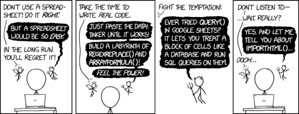
Figure 2. “Spreadsheets,” xkcd.com no. 2180.
MS Excel, Google Sheets, Apple Numbers, and for that matter, Calc, the spreadsheet application in my favorite office app LibreOffice (LibreOffice is a free, open-source alternative to Microsoft Office), can be used to calculate many descriptive statistics. With some effort, these applications can be extended by use of either Analysis ToolPak or Solver Add-ins to do more complicated statistics like regression and analysis of variance, and curve fitting.
Note 4. Perhaps you’re thinking: I’m a data science student — it’s not whether we chose between use of spreadsheet apps or R, we should be using Python, shouldn’t we? DrD — this is an open question, and if you judge the job market as the arbiter, I’d say learn Python over R — if you are primarily aiming for a data science position. However, from the point of view of learning statistics, my vote would be R — far more packages developed to accomplish our tasks, and, at least for this course, we are not teaching coding: our focus is on using statistics to explore (describe) and ask questions about data collected by observation or experimentation.
While we’re on the subject in 2025, it looks like the job market is in Machine Learning, which means R or Python knowledge will be a given, but advantage will go to those who know Alteryx or it’s open source alternative KNIME for data science workflow design — from data collection to model development.
However, use of MS Excel for statistical analysis involves learning a number of commands, syntax, and developing workflows that are neither intuitive nor standard. Some publishers have provided add-ins that are reportedly designed to simplify this process (eg, XLStat, UNISTAT, Real Statistics using Excel). None of these options are free and none are in use in any major way by scientists (see Robert Muenchen’s The popularity of data analysis software). The free add-ins of Analysis ToolPak and Solver may work for you if you own a Windows PC, but only Solver is included for the Mac versions of Excel. MacOS users may download and install StatPlus:MacLE, which is a limited, but free alternative to the Analysis ToolPak add-in; for a complete package a Pro version is available (licenses started at $89, web site: www.analystsoft.com/en/products/statplusmacle/).
An additional caution: you should be aware that there have been reports over the years that algorithms selected by Microsoft for Excel have not always been to industry standards (eg, McCullogh and Wilson 2005). In short, the fit of Excel and other spreadsheet apps for use in statistics is not a simple one. To do the kinds of statistics we will use routinely in class, Excel would need to be modified with add-ins, and the add-ins would be the result of programming by someone. And you would still need to learn how to write the code.
What about graphics? You may like Microsoft Excel’s ability to do graphics. Indeed, Excel, Google Sheets, and LibreOffice Calc can be used to generate many typical kinds of statistical plots. But again, in comparison to R, spreadsheet app graphics are limited and require a deal of effort to generate acceptable plots. I think you’ll be surprised at how straight-forward R is. Here’s an example, first rendered in Microsoft Excel, then in base R. And importantly, the kinds of plots Excel does well at are not necessarily the plots suitable for research publication. For example, Excel allows you to make bar charts easily, but cannot do box plots. Box plots are preferred over bar (column) charts for ratio scale data.
Note 5. base R refers to the core R programming language along with many functions and graphics routines. We extend capabilities of base R by adding packages, like R Commander.
Statistics comparisons between R and MS Excel.
.
About that learning curve. Let’s compare R and MS Excel for basic functions common in data analysis. Similar conclusions hold for comparisons to Google Sheets and LibreOffice Calcs.
Note 6. If you search for variants of this question, you’ll find other’s making the argument that the learning curve for many data science tasks is, perhaps surprisingly, shorter for R than it is for Excel. For example, see Amieroh Abrahams 2023 article at https://www.jumpingrivers.com/blog/comparing-r-excel-data-wrangling/ .
Table 2 lists the observations we can use to conduct comparisons of the applications.
A simple data set
| varA |
|---|
| 12 |
| 14 |
| 20 |
| 25 |
| 28 |
| 29 |
| 32 |
| 34 |
| 35 |
| 39 |
| 47 |
| 47 |
| 50 |
| 53 |
| 54 |
| 71 |
| 79 |
| 87 |
| 89 |
| 96 |
| 105 |
| 122 |
| 130 |
| 132 |
One of the first steps in data analysis is to produce what are called descriptive statistics. Common descriptive statistics are the mean and the sample standard deviation. Let’s compare Excel and R for retrieving these two statistics.
With Excel, to calculate the arithmetic mean of 24 numbers, enter the values into a single column of 24 rows, then enter “=average(A2:A25)“, without the quotes, into a new cell of the spreadsheet. “A2:A25” refers to where data would be contained in column A rows 2 through 25. Typically the first row in a worksheet would contain the name of the variable, eg, “A.” Depending on the significant figures set, the estimate returned by Excel for the mean of A is 59.58333333.
Similarly, to obtain the standard deviation, type =stdev(A2:A25), into a new cell of the spreadsheet. Again, depending on the significant figures set, Excel returns a value of 37.05215674 for the standard deviation of A.
In contrast, to obtain the mean and standard deviation for a variable in an R data set, all you would type at the R prompt (>), or in the script window
Note 7. Always run your code as a script. Entering code at the R prompt means you are working at the command-line interface, and you work one line at a time. This is not an efficient way to interact with R. Instead, I recommend you always create and work from a script document. For beginners, that’s why I recommend R Commander, which includes a script window. Simply type your code in the script window, highlight the code you wish to run, and run by clicking submit button (or Ctrl+R Win11 or Cmd+Enter macOS). When you are ready to move on from R Commander, RStudio is the IDE of choice.
and then submit the code is:
myA <- c(12, 14, 20, 25, 28, 29, 32, 34, 35, 39, 47, 47, 50, 53, 54, 71, 79, 87, 89, 96, 105, 122, 130, 132)where the “c” is a function to combine arguments into a vector and saved to the object myA, followed at the new line by
mean(myA)Hit enter after entering the command) and R returns
[1] 59.58333For the standard deviation, write the R base function sd()
sd(myA)Hit enter after entering the command and R returns
[1] 37.05216It’s not much of a difference, but note that to get the mean (arithmetic average) I typed seven characters in R, but 16 characters in Excel; similarly, for the standard deviation I typed in 5 characters in R, but 13 characters in Excel. That’s a savings of 56% and 62%, respectively. Excel tries to help by using AutoComplete to anticipate what you want to enter, but AutoComplete doesn’t always work properly (eg, see gene name errors generated by use of default Microsoft Excel settings, Ziemann et al 2016).
Note 8. I use spreadsheets all of the time for data entry and data management. Make sure AutoComplete and AutoCorrect options are turned off and these problems are much less.
In conclusion, R is quicker for descriptive statistics.
Graphics comparison between R and MS Excel.
.
MS Excel is often cited for its graphics capabilities (Camões 2016). We can make the familiar scatter plots, bar charts, and pie charts in Excel. These plots and more are easily obtained in R. I won’t elaborate here about graphics, we talk at some length about graphics in Chapter 4. But here’s one example in R.
Let’s plot myB vs myA. We already provided the data for variable A, here’s the data for variable B.
17, 21, 21, 26, 27, 32, 28, 42, 40, 30, 71, 53, 56, 61, 55, 89, 82, 63, 116, 162, 116, 154, 137, 149Don’t recall how to assign a set of numbers to an object, B, in R? See above and look again at how we assigned the numbers to object myA.
To get a simple scatter plot (Fig 3), I may write at the R prompt.
plot(myA,myB)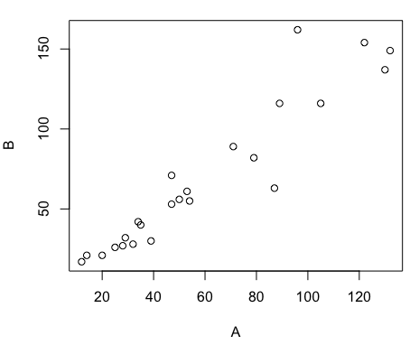
Figure 3. Basic scatter plot made in R, plot(myA,myB).
And here’s the comparable default plot (Fig 4) from Microsoft Excel, Office 365
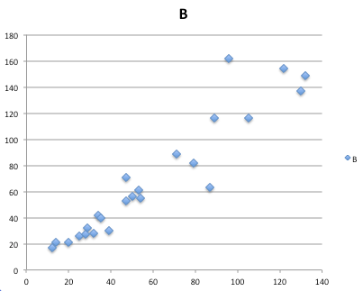
Figure 4. Basic scatterplot made in Microsoft Excel.
Now, both graphs need some work, and to be fair, these are just the defaults. With some effort, you can make an Excel graph look pretty good. But note — the defaults in Excel don’t generate axis labels, while R default plot does. Excel adds a useless title and legend; both need to be removed. Excel also adds grid lines where typically one would not include these in a scientific plot; for example, in the case of scatterplots, grid lines can distract the viewer from the data points and reduce the data-to-ink ratio Tufte 1984).
Count the steps to generate an acceptable scatter plot (Table 3). I’ve also added R Commander (Rcmdr) steps for comparisons (Rcmdr lets you use drop-down menus like Excel or Google Sheets or LibreOffice Calcs).
Table 3. Steps needed to make a simple scatterplot in R, R Commander, or Microsoft Excel.
| Steps | R | Rcmdr | Excel 365 |
| 1 | write the function | Select Graphs | Highlight columns |
| 2 | Select scatterplot | Select from Menu “Insert” | |
| 3 | Select variables | Select scatterplot | |
| 4 | Uncheck options | Select type of scatterplot | |
| 5 | Delete legend | ||
| 6 | Remove grids | ||
| 7 | Insert X-axis label | ||
| 8 | Insert Y-axis label |
Conclusion? R is quicker for routine statistical plots like a scatter plot. And I didn’t even count the steps needed to change MS Excel’s dreadful diamond icon points.
That’s one step in R, four steps in Rcmdr, but eight steps for Microsoft Excel. LibreOffice Calc is a little better at only four steps, but like MS Excel, you’d need to change several components to the graph (Fig 5).
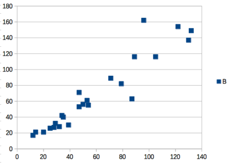
Figure 5. Basic scatterplot made in LibreOffice Calc.
Note 9. In R vernacular, these are referred to as pch, or point characters: pch = 23 returns a blue diamond character; for a blue square like Figure 5, add to the plot() command as
plot(myA,myB, pch = 22)
So, you’re telling me I don’t need a spreadsheet application?
.
No, not at all. We use spreadsheets, and more generally, databases, to store data. Spreadsheets apps are designed to make data entry and data management approachable and efficient. They remain an important tool for researchers (Browman and Woo 2017).
R is not that great of a spreadsheet; packages are available to seamlessly tie your spreadsheet and database data to R via ODBC. We will routinely enter and manipulate data in MS Excel, then import the data into R for analysis.
Spreadsheet apps like MS Excel and Google Sheets (see also LibreOffice Calc) are great at being a spreadsheet program, R is great at being a statistical software program. You should take advantage of what the tools do best.
Still not convinced?
.
R is in use all over the world, by students and professionals alike and if one is going to spend the time to learn how to use a statistics software program, you should learn a standard program, like R.
And it’s not just me. Read about R in this 2009 New York Times piece, “Data analysts captivated by R’s power.” Look who purchased (April 2015) Revolution Analytics, a major player in the development of the R programming language.
Note 10. The answer was Microsoft. For several years Microsoft supported R development via Microsoft Machine Learning Server & Microsoft R Open. However, as of July 2023, this service is no longer available. See Microsoft R application network retirement.
Why install R on your computer?
.
Convenience. Control. Offline.
At the Biology department of Chaminade University, we have installed and maintain R, Rcmdr, and RStudio along with all required packages on our Macbook Pro® Lab computers for your use during class and during optional, proctored biostatistics work sessions. Since 2018, R is increasingly available “in the cloud” (eg, RStudio Cloud), which would mean you could run R in your browser and avoid installation on your computer. You can run significant analysis with R in the cloud via the free Google Colaboratory and CoCalc are now available: I encourage you to look into these platforms. Unfortunately, these services are not quite ready for the classroom. For example, RStudio in the Cloud is free to use on a limited basis, but quickly requires a significant subscription cost with increasing use. Google Colab and GoCalcs require use of Jupyter notebooks, which add yet another layer to the learning curve without focusing on learning statistics. Second, although access to their servers is easy, running simultaneous connections via Chaminade’s single public IP address is likely to lead to problems for us. Third, I want you to use R Commander (Rcmdr) to assist in the learning curve — Rcmdr cannot be run in the Cloud (ie, RStudio in the Cloud, Google Colaboratory, or CoCalc).
Therefore, you are encouraged to install R, Rcmdr, and even RStudio, onto your own computers, in part because of the convenience, but also because R is not generally available to students on campus, ie, only the Biology department’s computers have the up-to-date R software installed.
To get started, go to your Canvas website and view How to install R on your own computer.
An additional benefit to installing a version of R on your computer, you’ll understand more about the software if you take the time to install and if need be, troubleshoot your installation of the software. Moreover, there’s a considerable amount of help out there for R. For example, a simple Google search(keywords: tutorial “install R”), returns more than 700K hits, and more than 40K January 2023 alone (add “after:2023-01-01” to Google search box). In fact, there’s so much out there that you’ll want to sample from several sites and select the voice that works best for you.
Questions
- Write up three learning outcomes for this page. Hint: Point your favorite generative AI to this page and ask for help.
- I listed several spreadsheet apps: Microsoft Excel, Google Sheets, Apple Numbers, LibreOffice Calc. Which of these are free to download and install to your computer? Which are freely available via the Cloud?
- What level of confidence do you have to this statement: I am confident in my ability to use spreadsheet apps for my BI-311 work this semester. Response options:
- Strongly disagree.
- Disagree.
- Agree.
- Strongly agree.
- What level of confidence do you have to this statement: I am confident in my ability to use the R programming software for my BI-311 work this semester. Response options:
- Strongly disagree.
- Disagree.
- Agree.
- Strongly agree.
.
Quiz Chapter 2.2
Why do we use R software?
Chapter 2 contents
.
1.1 – A quick look at R and R Commander
A first look at R.
R is a programming language for statistical computing (Venables et al 2009). R is an interpreted language — when you run (execute) an R program — the R interpreter intercepts and runs the code immediately through its command-line interface, one line at time. Python is another popular interpreted language common in data science. Interpreted languages are in contrast to compiled languages, like C++ and Rust, where program code is sent to a compiler to a machine language application. R is free to use and available via many platforms, from local installations on a person’s laptop to running on cloud servers (Fig 1). 
Figure 1. Choose how you will interact with R: on your computer (Blue box) or in the cloud (Red box). Users of Linux, macOS, and WinPC can either install R to their computer or choose to access R in the cloud (and/or, black arrow).
Before you begin, you have a choice: how do you want to work with R (Fig 1)? In part, the choice depends on your computing device. If you have a desktop or laptop computer, running Linux, Apple macOS, or Microsoft Windows, then R can be installed onto your computer (blue box, Fig 1). If, however, you have a ChromeBook, Apple iPad or iPhone, or any Android Tablet or Smartphone, you would go with the second option (red box, Fig 1).
For those going with installing R to their computer, the second choice is to pick the environment for creating and running scripts and managing file input and output during a session. Working environments for R in the cloud include RStudio and Jupyter Notebooks (eg, Google CoLab) (red box, Fig 1 — see Note 2 below). For installed R, two suggested environments are R Commander and RStudio, an Integrated Development Environment or IDE, RStudio (Fig 1). The choice depends on your needs — an IDE is helpful when you plan to write a lot of code, it’s a comprehensive programming environment, which includes many tools that support writing code from scratch.
For our course at Chaminade University, I recommend R Commander because of the drop-down menu approach to accessing statistical functions in R; R Commander is not a comprehensive environment, but it provides the necessary scripting window along with access to markdown editing. R Commander, Rcmdr, is an R package that provide a graphical user interface or GUI for R. It is based on the tcltk package. R must be installed first before installing the R Commander package. R Commander provides familiar menu functions, like many commercial statistical software. R Commander, like the IDE RStudio, is not necessary for R programming or conducting statistical analysis or even generating reports via markdown. R Commander, however, shrinks the learning curve with R programming basics so that students can focus on learning statistics, which is the chief objective of the Biostatistics course at Chaminade.
The following steps user through use of R and R Commander, from installation to writing and running commands. Mike’s Workbook for Biostatistics has a ten-part tutorial, A quick look at R and R Commander, which I recommend.
Note 1: Getting started? By all means rely on Mike’s Biostatistics Book (Appendix: Install R, Install R Commander, Use R in the cloud) and blogs or other online tutorials to point you in the right direction. You’ll also find many free and online books that may provide the right voice to get you working with R. However, the best way to learn is to go to the source. The R team has provided extensive documentation, all included as part of your installation of R. In R, run the command RShowDoc("doc name"). replace doc name with the name of the R manual or R user guide. For example, the Venables publication is accessed as RShowDoc("R-intro"). Similarly, the manual for installation is RShowDoc("R-admin") and the manual for R data import/export is RShowDoc("R-data").
Install R.
.
Full installation instructions are available at Install R, and for the R Commander package, at Install R Commander. Here, we provide a brief overview of the installation process.
Note 2: The instructions at Mike’s Biostatistics Book assume use of R on a personal computer running updated Microsoft Windows or Apple macOS operating systems. For Linux instructions, eg, Ubuntu distro, see How to install R on Ubuntu 22.04. For Chromebook users, if you can install a Linux subsystem, then you can also install and run R although it’s not a trivial installation. For instructions to install R see Levi’s excellent write up at levente.littvay.hu/chromebook/. (This works best with Intel-based CPUs — see my initial attempts with an inexpensive Chromebook at Install R.)
Another option is to run R in the cloud via service like Google’s Colab or CoCalc hosted by SageMath. Both support Jupyter Notebooks, a “web-based interactive computational environment.” Neither cloud-based service supports use of R Commander (because R Commander interacts with your local hardware). Colab is the route I’d choose if I don’t have access to a local installation of R. See Use R in the cloud for more details.
Download a copy of the R installation file appropriate for your computer from one of the Comprehensive R Archive Network (CRAN) mirror site of the r-project.org. For Hawaii, the most convenient mirror site is provided by the folks at RStudio (https://cloud.r-project.org/. In brief, Windows 11 users download and install the base distribution. MacOS users must first download and install XQuartz (https://Xquartz.org), which provides the X Window System needed by R’s GUI (graphic user interface). Once XQuartz is installed, proceed to install R to your computer. MacOS users — don’t forget to drag the R.app to your Applications folder!
Start R.
.
The following is a minimal look at how to use R and R Commander. Please refer to tutorials at Mike’s Workbook for Biostatistics (R work, part 1 – 10) to learn use of R and R Commander.
We’re just getting started, so the next thing to learn is how to set your working environment for your R sessions. Although we’ll discuss the R environment more as we proceed, it’s a good idea to start with a best practice action common in data science — always create and work from a working folder. This can be a local folder on your computer or pointed to a folder in your cloud storage. On my mac I usually create a folder on the desktop, example BI-311, and point to that as my working folder for a project. Now, we need to point R to use the working folder — we do this at start of each R session (or modify some code R needs during start up to always point to the folder — for now, we leave that for a later exercise).
Once R is installed on your computer, start R as you would any program on your computer. For example, the icon for the R.app as it appears in the dock on a MacBook is shown in Figure 2.

Figure 2. R.app icon shown on a MacBook dock.
To point R to our working folder, there are several options. For now, we’ll go with writing and submitting a simple function in R. Recall that R has a command-line. The R prompt appears on the command line in the RGUI as the greater-than typographical symbol “>” at the beginning of a line (Fig 2). The prompt is returned by R to indicate the interpreter is ready to accept the next line of code.
First, discover where R is pointing to by submitting (type the command exactly as written then select keyboard shortcuts on Windows enter, or on macOS return key) the function getwd() at the prompt.
Note 3: Unfamiliar with keyboard shortcuts? I created a page just for you at Keyboard shortcuts in Mike’s Workbook for Biostatistics.
Ready to
On my MacBook, R returns
> getwd()
[1] "/Users/[username]/Documents"
To point to my working folder, I submit setwd("/Users/[username]/Desktop/BI311". When I run getwd() again, R returns the update
> getwd()
[1] "/Users/[username]/Desktop/BI311"
Note 4: Windows users will recognize that, unlike macOS and Linux, they will need to write paths with the backslash, not the forward slash. This is discussed further in Mike’s Workbook.
[username] is just a placeholder here — no reason to share my actual user name!
Ready to do some work?
R coding practices in this book and in the companion workbook roughly follow guidance outlined in a September 2018 R-Bloggers post, “R Code — Best practices,” by The R Trader. Of note, naming conventions: variables are nouns, variable names are written in lowerCamelCase; functions are verbs, function names are period separated, eg, my.function; script file names all end with .R and are written snake_case.R. Comments, preceded by # and a single space, eg, # A brief comment, are sparingly included in code, but reserved for explanatory sentences in the text. We use <- and not = for assignment statements.
Where discussion requires reference to instructions on use of the R programming language, R code (instructions) the user needs to enter at the R prompt are shown in code blocks.
Courier New font within a “code block.”Until you write your own functions, the general idea is, you enter one set of commands at a time, one line at a time. For example, to create a new variable, curryPoints, containing points scored by the NBA’s Steph Curry during the 2016 playoffs, type the following code at the R prompt (displayed as >, the “greater than” sign)
curryPoints <- c(24,6,40,29,26,28,24,19,31,31,11,18,19).
and to obtain the mean, or arithmetic average, for curryPoints at the R prompt type and enter
.
mean(curryPoints).
Output from R function mean will look like the following
.
[1] 24.42857.
Functions in R, or any other data science programming language, are intended to automate a task.
Note 5: A good data management habit — store the variable as an R object called a data.frame.
df.curryPoints <- data.frame(curryPoints)
The R prompt appears in the RGUI as the greater-than typographical symbol “>” at the beginning of a line (Fig 3). The prompt is returned by R to indicate the interpreter is ready to accept the next line of code.
![Screenshot of the R GUI on a macOS system; red arrow points to the R prompt. The visible code reads curry.points and some numbers between parentheses, next line calls for the mean of the object, and the last line begins with [1] and the result.](https://biostatistics.letgen.org/wp-content/uploads/2020/09/RGUI_prompt.png "Figure 1. The R GUI on a macOS system; red arrow points to the R prompt.")
Figure 3. The R GUI on a macOS system; red arrow points to the R prompt.
Note 6: We just demonstrated one of several ways data can be brought into an R session, by creating a data.frame directly from a vector. Other methods include
- Reading a text file from your computer, eg, CSV, by
read.csv() - Importing a spreadsheet (Excel file) from your computer
using readxl::read_excel() - Entering small datasets directly using
read.table()with thetext= argument
Everything that exists is an object.
.
A brief programmer’s note — John M. Chambers, creator of the S programming language and a member of the R-project team, once wrote that sub-header phrase about R and objects. What that means for us: programming objects can be a combination of variables, functions, and data structures. During an R session the user creates and uses objects. The ls() function is a useful R command to list objects in memory. If you have been following along with your own installed R app, then how many objects are currently available in your session of R? Answer by submitting ls(). Hint: the answer should be one object.
A routine task during analysis is to calculate an estimate then use the result in subsequent work. For example, instead of simply printing the result of mean(curryPoints), we can assign the result to an object.
myResult <- mean(curryPoints)
.
To confirm the new object was created, try ls() again. And, of course, there’s no particular reason to use the object name, myResult, I provided! Like any programming language, creating good object names will make your code easier to understand.
When you submit the above code, R returns the prompt, and the result of the function call is not displayed. View the result by submitting the object’s name at the R prompt, in this case, myResult. Alternatively, a simple trick is to string commands on the same line by adding ; (semicolon) at the end of the first command. For example,
myResult <- mean(curryRoints); myResult
.
Objects created during an R session, like curryPoints, are stored in memory within the Global Environment. To remove an object, use the command rm(myVariable). Why remove objects during an R session? If you are attempting multiple tasks in a homework assignment, removing unneeded objects helps maintain a clean and organized workspace, improving code readability and reducing the chance of accidental errors.
Write your code as script.
.
While it is possible to submit code one line at a time, a much better approach is to create and manage code in a script file. A script file is just a text file with one command per line, but potentially containing many lines of code. Script files help automate R sessions. Once the code is ready, the user submits code to R from the script file.
Note 7: Working with scripts eliminates the R prompt, but code is still interpreted one line at a time. The user does not type the prompt in a script file.
Figure 4 shows how to create a new script file via the RGUI menu: File → New script.

Figure 4. Screenshot of drop down menu RGUI, create new script, Windows 11.
The default text editor opens (Fig 5).

Figure 5. Screenshot of portion of R Script editor, Windows 11. A simple R command is visible.
Submit code by placing cursor at start of the code or, if code consists of multiple lines, select all of the code, then hit keyboard keys Ctrl + R (Windows 11) or for macOS, Cmd + Enter.
I recommend starting with a clean environment, by using rm(list = ls()) at the beginning of a script.
By default, save R script files for reuse with the file extension .R, eg, my_script.R. Because the scripts are just text files you can use other editors that may make coding more enjoyable (see RStudio in particular, but there are many alternatives, some free to use. A good alternative is ESS).
Install R Commander package.
.
By now, you have installed the base package of the R statistical programming language (see for detailed instructions). The base package contains all of the components you would need to create and run data analysis and statistics on sets of data. However, you would quickly run into the need to develop functions, to write your own programs to facilitate your work. One of the great things about R is that a large community of programmers have written and contributed their own code; chances are high that someone has already written a function you would need. These functions are submitted in the form of packages. Throughout the semester we will install several R packages to extend R capabilities. R packages discussed in this book are listed at R packages of the Appendix.
Our first package to install is R Commander, Rcmdr for short. R Commander is a package that adds function to R; it provides a familiar point-and-click interface to R, which allows the user to access functions via a drop-down menu system (Fox 2017). Thus, instead of writing code to run a statistical test, Rcmdr provides a simple menu driven approach to help students select and apply the correct statistical test. R Commander also provides access to Rmarkdown and a menu approach to rendering reports.
install.packages("Rcmdr")
.
In addition, download and install the plugin
install.packages("RcmdrMisc")
See Install R Commander for detailed installation instructions.
Note 8: Plugins are additional software which add function to an existing application.
Start R Commander.
.
After installing Rcmdr, to start R Commander, type library(Rcmdr) at the R prompt and enter to load the library
library(Rcmdr).
On first run of R Commander you may see instructions for installing additional packages needed by R Commander. Accept the defaults and proceed to complete the installation of R Commander. Next time you start R commander the start up will be much faster since the additional packages needed by R Commander will already be present on your computer.
Note that you don’t type the R prompt and, indeed, in R Commander Script window you won’t see the prompt (Fig 6). Instead, you enter code in the R Script window, then click “Submit” button (or Win11: Ctrl+R or for macOS: Cmd+Enter), to send the command to the R interpreter. Results are sent to Output window (Fig 6).
 Rcmdr ver. 2.4-4.")
Figure 6. The windows of R Commander, macOS. From bottom to top: Messages, Output, Script (tab, Markdown) Rcmdr ver. 2.4-4.
Figure 6 shows how the R Commander GUI looks on a macOS computer. The look is similar on Microsoft Windows 11 machines (Fig 7).
 Rcmdr ver. 2.5-1.")
Figure 7. The windows of R Commander, Win11. From bottom to top: Messages, Output, Script (tab, R Markdown) Rcmdr ver. 2.5-1.
We use R Commander because it gives us access to code from drop-down menus, which at least initially, helps learn R (Fox 2005, Fox 2016). Later, you’ll want to write the code yourself, and RStudio provides a nice environment to accomplish your data analysis.
Improve Rcmdr experience.
Windows users: R Commander works best in Windows if SDI option is set. This can be accomplished during R installation (“Startup options” popup, change from default “No” to “Yes” to customize), but you can also change after installing R. Win11 users should change from MDI to SDI — from one big window to separate windows — (see Do explore settings, WinPC see Fig 9; macOS see Fig 10). The downside of SDI is that while multiple Windows may appear during an R session, one or more windows may be hidden by an open window. For example, plots will popup in a new window and may be obscured by the Rcmdr window if full screen. A simple trick to view active windows on Win11 is to use the keyboard shortcut s Alt + Tab to view and cycle between windows. What about SDI and RStudio? RStudio experience will be similar whether MDI (default) or SDI was selected.
macOS users: To improve R Commander performance, turn off Apple’s app nap (see Do explore settings, Figures 6), which should improve a Mac user’s experience with R Commander and other X Window applications.
Complete R setup by installing LaTeX and pandoc for Markdown.
.
LaTeX is a system for document preparation. pandoc is a document converter system. Markdown is a language used to create formatted writing from simple text code. Once these supporting apps are installed, sophisticated reports can be generated from R sessions, by-passing copy and paste methods one might employ. See Install R Commander for instructions to add these apps.
Note 9: If you successfully installed R and are running R Commander, but may be having problems installing pandoc or LaTeX, then this note is for you. While there’s advantages to getting pandoc etc working, it is not essential for BI311 work.
Assuming you have Rcmdr and RcmdrMisc installed, and if you have started Rcmdr and have it up and running, then we can skip pandoc and LaTeX installation and use features of your browser to save to pdf.
R Markdown by default will print to a web page (an html document called RcmdrMarkdown.html) and display it in your default browser. To meet requirements of BI311 — you submit pdf files — we can print the html document generated from “Generate Report” in R Commander to a pdf.
- Chrome browser, right click in the web page, from the popup menu select Print, then change destination to Save as pdf.
- Safari browser, right click then select Print page (or if an option, Save page as pdf), then find at lower left find PDF and option to Save as PDF.
R Markdown.
.
Markdown is a syntax for plain text formatting and is really helpful for generating clean html (web) files. R Commander also helps us with our reporting. R Markdown is provided as a tab (Fig 6, Fig 7). Provided you have also installed pandoc on your computer, you can also convert or “render” the work into other formats including pdf and epub. Unsure if your computer has pandoc installed? If you are unsure than most likely it is not installed. 😁 Rcmdr provides a quick check — go to Tools and if you see Install auxiliary software, then click on it and a link to pandoc website to find and download installation file. You can also confirm install of pandoc by opening a terminal on your computer (eg, search “terminal” on macOS or “cmd” on Win11), then enter pandoc –version at the shell prompt. Figure 8 shows version pandoc is installed on my Win11 HP laptop.
 on win11 computer, checking for installed pandoc on a win10 pc.")
Figure 8. Screenshot of terminal window (cmd) on win11 computer, checking for installed pandoc on a win10 pc.
Enter your R code in the script window, submit your code, and your results (code, output, graphs) are neatly formatted for you by Markdown. Once the Markdown file is created in R Commander, you can then export to an html file for a a web browser, an MS Word document, or other modes.
Do explore settings!
.
After installation, R and R Commander are ready to go. However, students are advised that a few settings may need to be changed to improve performance. For example, on Win11 PCs, R Commander recommends changing from the default MDI (Multiple Document Interface) to SDI (Single Document Interface). Check the SDI button via Edit menu, select GUI preferences menu. Click save, which will make changes to .RProfile, then exit and restart R. Check to make sure the changes have been made (Fig 9).

Figure 9. Screenshot of GUI preferences settings after changing from default MDI to SDI, win10
For macOS users, both R and Rcmdr will run better if you turn off Apple’s power saving feature called nap. From Rcmdr go to Tools and select Manage Mac OS X app nap for R.app… (Fig 10).

Figure 10. Screenshot Rcmdr Tools popup menu, macOS 10.15.6
A dialog box appears; select off to turn off app nap (Fig 11).

Figure 11. Screenshot Rcmdr Set app nap dialog box, macOS 10.15.6
Exit R Commander.
.
Click on Rcmdr: File → Exit, then choose to exit from just R Commander, or both R Commander and R.
If you exit just R Commander or both R and R Commander, you’ll receive a pop-up request to confirm you want to quit R Commander (click yes), and a second prompt asking if you want to save your script. In general, select yes and then you’ll be able to take up where you left off. Similarly, if asked to save your workspace, choose no. If you save workspace, this creates an .RProfile text file with settings for how R and R Commander will behave the next time you start R. The file will be saved to your current working folder, which R will use the next time R starts. At least while you are getting started, you should avoid creating these .RProfile files.
As long as the current session of R is active, then the library for Rcmdr, as well as any other library loaded during the R session, is in memory. To start R Commander again while R is running, at the R prompt, type and submit
Commander()
Questions.
- Biostatistics students should work through my ten R lessons, A quick look t R and R Commander, available in Mike’s Workbook for Biostatistics.
- Students should also search Internet for R tutorials and R Commander tutorials. Find recent tutorials and work through several of them. We get better when we practice.
Quiz Chapter 1.1
A quick look at R and R Commander
Chapter 1 contents
.
- Getting started
- A quick look at R and R Commander
- Chapter 1 – References
Mike’s Biostatistics Book
.")
Mike’s Biostatistics Book is an eBook to support my Biostatistics course at Chaminade University (since 2009). The course had its origins at the University of Hawaiʻi at Hilo (2003 – 2005), and was inspired by a course of the same name taught by Don Price (now at UNLV). The progression and structure of this ebook follows my presentation in the course — BI-311 Biostatistics — these are my extended lecture notes. The companion site, Mike’s Workbook for Biostatistics, provides homework and simple projects to learn-by-doing biostatistics.
In September 2024, Mike’s Biostatistics Book was adopted LibreTexts.org for inclusion in their open textbook applied statistics library.
Mike’s Biostatistics Book is a work in progress; some chapters are complete, others, not so much. With each semester I add to and rewrite content. The draft of this eBook adopted by LibreTexts in Fall 2024 is at the level of version 0.99; We may as well then refer to this release of the book as version 1+.
The BI311 course is typically offered in Fall semester; following the semester I update the text. Thus, since Fall 2024 I’ve added content, and since September 2024 I added several subchapters, added text to more than 50% of the pages, and have updated the book with proof-reading for typos, clarity and organization flow, a more complete index page to key words and a complete listing of all 400+ figures contained in the book. So far in Fall 2025, I updated instructions on use of R in Jupyter Notebooks and the cloud. New in Fall 2025, I’ve added about 900(!) true/false or multiple choice questions with immediate feedback — correct or incorrect — to accompany each subchapter. I have yet to complete a couple of sub-chapters in Chapter 19 and Chapter 20.
Thus, post LibreText.org adoption, this version of Mike’s Biostatistics Book hosted at my website is 1.89. Why not round to two? Let’s introduce our first statistics concept — precision. Because I’m not following a proscribed version control scheme eg, Git, there can be no claim that “1.89” is precise — that is, exact to the hundredths. We may as well then refer to this release of the book as version 2+.
The cover image is a manowar fractal (now called “leaves” in 3.0.4 GIMP) generated in Fractal Explorer, the GNU Image Manipulation Program (GIMP).
Text to speech — Google US English — is provided by WordPress plugin Text To Speech TTS Accessibility, free version.
Fall 2025
/MD
2 – Introduction
Why biostatistics, not “biometry”?
.
Chapter 1 – Getting started, we presented a brief introduction to statistical thinking, a systematic approach to how we ask questions about the world from data. The chief learning objective of this eBook, then, is to provide the reader with a framework and practical computing skills needed for statistical reasoning in the biological sciences. Chapter 1 – Getting started also offered a justification for why undergraduate biology students should (are required) learn (bio)statistics. In my day, most of us took statistics as part of our graduate training. The curriculum for science students has accelerated now — it is now assumed that as part of undergraduate career students gain experience working with data and developing quantitative reasoning skills. Biostatistics courses are designed to help you achieve this understanding. We expand on that point in Ch2.1 – Why biostatistics?.
Note 1: I took a business statistics class as an undergraduate student at the University of Washington in the early 1980s. The textbook was the 6th edition of John E. Freund‘s Modern Elementary Statistics. Biostatistics course was not an option for a biology undergraduate student at the time. During my first year of graduate school at the University of Wisconsin, textbooks were the 2nd edition of Biometry by Robert R. Sokal and F. James Rohlf) and the 8th edition of Statistical Methods by G.W. Snedecor and W.G. Cochran.
Biostatistics generally refers to the application of statistical methods to biological research in the context of medicine and public health. The emphasis of biostatistics is on experimental design and hypothesis testing in clinical and epidemiological contexts. The term biostatistics first appears in the literature in the 1940s (Pubmed). On the other hand, biometry, sensu the title of Sokal and Rohlf‘s legendary textbook, is a broader term, associated with the application of mathematical and statistical techniques to biological problems, especially in fields like ecology, genetics, and evolution. Our eBook provides real world problems as examples from across the biological field, including agriculture, ecology, evolution, genetics as well as health topics, thus the subject of this text is more in line with the spirit of biometry. However, I titled the book “Mike’s Biostatistics Book,” not “Mike’s Biometry Book,” because the term biometry is now conflated with biometrics (Oxford English Dictionary), which refers to the technology used to identify individuals based on biological characteristics.
Chapter 2 begins my sales pitch: Why biostatistics? We’ll also provide a selective history of biostatistics and how statistical thinking informs the design of experiments. Chapter 2 concludes with how statistical reasoning fits in the scientific method — the systematic approach to acquiring knowledge through observation, experimentation, and reasoning (Chapter 2.5) — and introduces project-based learning approaches used in the biostatistics course at Chaminade University.
Quizzes in this chapter
A total of 50 questions among the several subchapters, a mix of true or false and multiple choice question format.Homework to go with this topic.
Homework 1: Project data life cycle in Mike’s Workbook for Biostatistics.
Chapter 2 contents
.
- Introduction
- Why biostatistics?
- Why do we use R Software?
- A brief history of (bio)statistics.
- Experimental Design and rise of statistics in medical research.
- Scientific method and where statistics fits.
- Statistical reasoning.
- Chapter 2 – References and suggested reading.
0.1 – Disclaimers and copyright
Disclaimers
.
Because this is a biostatistics book, many of the examples and problems come from the medical and biomedical research literature. Nothing in this eBook, or included as part of any accompanying text, web site, or supplemental material to this eBook, should be construed as an attempt to offer or render a medical opinion or otherwise engage in the practice of medicine. I may be a doctor, but I’m not that kind of doctor.
Financial and opinion disclaimers
This site is solely supported by me, Michael “Mike” Dohm, and I don’t monetize the site. Responsibility for the content rests with me, not my employer, Chaminade University of Honolulu. The opinions expressed on this website, or supplemental material to this website, are solely those of the myself and do not necessarily reflect the views of my employer. Chaminade University is not responsible for any errors or omissions in this content or any damages resulting from its use.
Trademark Notice
.
Product or corporate names may be trademarks or registered trademarks, and are used only for identification and explanation without intent to infringe or endorse. A partial listing of products mentioned or discussed in this book include the following.
Copyright of the R statistical programming language is held by the R Foundation. R and R Commander are freely available under the GNU General Public License.
Markdown is registered trademark held by John Gruber.
Posit, Rstudio, R markdown, and Shiny are registered trademarks of Posit.
pandoc is the registered trademark held by Dr John MacFarlane.
Microsoft Access, Excel, Word, Microsoft Office, OneDrive, Windows, Windows XP, Windows Vista, Windows 8, Windows 10, and Windows 11 are registered trademarks of Microsoft Corporation.
Finder, iCloud, iPad, iPhone, macOS, Mac OS X, MacBook, MacBook Pro, OS X, Pages, Quartz, QuickTime, and Safari are registered trademarks of Apple Corporation.
LibreOffice is a registered trademark of The Document Foundation.
Chrome, Chromebook, Google Sheets,Google CoLaboratory, Google Docs, Google Drive are registered trademarks of Google LLC.
I have included several cartoons (n = 10) from the wonderful xkcd.com series by Randall Munroe. Copyright clearly belongs to xkcd.
Other products mentioned in this eBook are the trademarks of their registered owners.
No-responsibility disclaimer
.
Coding examples are provided throughout this eBook. No warranty applies; use of any code examples from this eBook and the “use at your own risk” liability disclaimer applies. The author shall not be liable for any loss of data or other direct or indirect losses that may or may not result from use of code presented herein.
Fair use disclaimer
All efforts to cite and reference scholarly works as needed are included, but there may be some content that may inadvertently refer to works not authorized by the copyright holder. However, Mike’s Biostatistics Book falls under Section 107 of the Copyright Act because it is intended for educational purposes only.
Copyright![]()
.
![]()
This work is licensed under a Creative Commons Attribution-NonCommercial-ShareAlike 4.0 International License.
How to cite this work
If you wish to use this material, please cite as Dohm, Michael R (2025) Mike’s Biostatistics Book version 2.0, biostatistics.letgen.org. The eBook does contain my attempt at evidence-based opinion on many statistics subjects. However, as the work is not peer-reviewed, and, like most textbooks, is predominately a secondary source, I would not recommend the eBook as a sole-source reference.
Preface contents
.
0.1 – Disclaimers and copyright