18.1 – Multiple Linear Regression
Introduction
Last time we introduced simple linear regression:
- one independent X variable
- one dependent Y variable.
The linear relationship between Y and X was estimated by the method of Ordinary Least Squares (OLS). OLS minimizes the sum of squared distances between the observed responses,  and responses predicted
  by the line. Simple linear regression is analogous to our one-way ANOVA — one outcome or response variable and one factor or predictor variable (Chapter 12.2).
But the world is complicated and so, our one-way ANOVA was extended to the more general case of two or more predictor (factor) variables (Chapter 14). As you might have guessed by now, we can extend simple regression to include more than one predictor variable. In fact, combining ANOVA and regression gives you the general linear model! And, you should not be surprised that statistics has extended this logic to include not only multiple predictor variables, but also multiple response variables. Multiple response variables falls into a category of statistics called multivariate statistics.
Like multi-way ANOVA, multiple regression is the extension of simple linear regression from one independent predictor variable to include two or more predictors. The benefit of this extension is obvious — our models gain realism. All else being equal, the more predictors, the better the model will be at describing and/or predicting the response. Things are not all equal, of course, and we’ll consider two complications of this basic premise, that more predictors are best; in some cases they are not.
However, before discussing the exceptions or even the complications of a multiple linear regression model, we begin by obtaining estimates of the full model, then introduce aspects of how to evaluate the model. We also introduce and whether a reduced model may be the preferred model.
R code
Multiple regression is easy to do in Rcmdr — recall that we used the general linear model function, lm(), to analyze one-way ANOVA and simple linear regression. In R Commander, we access lm() by
Rcmdr: Statistics → Fit model → Linear model
You may, however, access linear regression through R Commander
We use the same general linear model function for cases of multi-way ANOVA and for multiple regression problems. Simply enter more than one ratio-scale predictor variable and boom!
You now have yourself a multiple regression. You would then proceed to generate the ANOVA table for hypothesis testing
Rcmdr: Models → Hypothesis testing → ANOVA tables
From the output of the regression command, estimates of the coefficients along with standard errors for the estimate and results of t-tests for each coefficient against the respective null hypotheses for each coefficient are also provided. In our discussion of simple linear regression we introduced the components: the intercept, the slope, as well as the concept of model fit, as evidenced by R2, the coefficient of determination. These components exist for the multiple regression problem, too, but now we call the slopes partial regression slopes because there are more than one.
Our full multiple regression model becomes

where the coefficients β1, β2, … βn are the partial regression slopes and β0 is the Y-intercept for a model with 1 – n predictor variables. Each coefficient has a null hypothesis, each has a standard error, and therefore, each coefficient can be tested by t-test.
Now, regression, like ANOVA, is an enormous subject and we cannot do it justice in the few days we will devote to it. We can, however, walk you through a fairly typical example. I’ve posted a small data set diabetesCholStatin at the end of this page. Scroll down or click here. View the data set and complete your basic data exploration routine: make scatterplots and box plots. We think (predict) that body size and drug dose cause variation in serum cholesterol levels in adult men. But do both predict cholesterol levels?
Selecting the best model
We have two predictor variables, and we can start to see whether none, one, or both of the predictors contribute to differences in cholesterol levels. In this case, both contribute significantly. The power of multiple regression approaches is that it provides a simultaneous test of a model which may have many explanatory variables deemed appropriate to describe a particular response. More generally, it is sometimes advisable to think more philosophically about how to select a best model.
In model selection, some would invoke Occam’s razor — given a set of explanations, the simplest should be selected — to justify seeking simpler models. There are a number of approaches (forward selection, backward selection, or stepwise selection), and the whole effort of deciding among competing models is complicated with a number of different assumptions, strengths and weaknesses. I refer you to the discussion below, which of course is just a very brief introduction to a very large subject in (bio)statistics!
Let’s get the full regression model
The statistical model is

As written in R format, our model is ChLDL ~ BMI + Dose + Statin.
Note that BMI is ratio scale and Statin is categorical (two levels: Statin1, Statin2). Dose can be viewed as categorical, with five levels (5, 10, 20, 40, 80 mg), interval scale, or ratio scale. If we are make the assumption that the difference between 5, 10, up to 80 is meaningful, and that the effect of dose is at least proportional if not linear with respect to ChLDL, then we would treat Dose as ratio scale, not interval scale. That’s what we did here.
We can now proceed in R Commander to fit the model.
Rmdr: Statistics → Fit models → Linear model
How the model is inputted into linear model menu is shown in Figure 1.
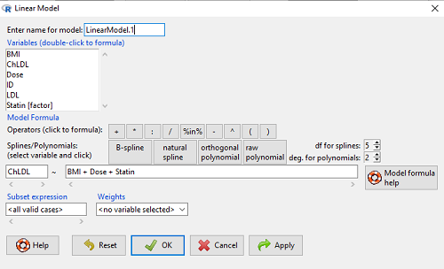
Figure 1. Screenshot of Rcmdr linear model menu with our model elements in place.
The output
summary(LinearModel.1)
Call:
lm(formula = ChLDL ~ BMI + Dose + Statin, data = cholStatins)

Residuals:
    Min      1Q  Median     3Q    Max
-3.7756 -0.5147 -0.0449 0.5038 4.3821

Coefficients:
                      Estimate Std. Error t value Pr(>|t|)
(Intercept)           1.016715   1.178430   0.863 0.39041
BMI                   0.058078   0.047012   1.235 0.21970
Dose                 -0.014197   0.004829  -2.940 0.00411 **
Statin[Statin2]       0.514526   0.262127   1.963 0.05255 .
---
Signif. codes: 0 '***' 0.001 '**' 0.01 '*' 0.05 '.' 0.1 ' ' 1

Residual standard error: 1.31 on 96 degrees of freedom
Multiple R-squared: 0.1231, Adjusted R-squared: 0.09565
F-statistic: 4.49 on 3 and 96 DF, p-value: 0.005407
Question. What are the estimates of the model coefficients (rounded)?
 = intercept = 1.017
 = slope for variable BMI = 0.058
 = slope for variable Dose = -0.014
 = slope for variable Statin = -0.515
Question. Which of the three coefficients were statistically different from their null hypothesis (p-value < 5%)?
Answer: Only coefficient was judged statistically significant at the Type I error level of 5% (p = 0.0041). Of the four null hypotheses we have for the coefficients:
 = 0
= 0 = 0
= 0 = 0; we only reject the null hypothesis for
 Dosecoefficient. = 0)
= 0)
Note the important concept about the lack of a direct relationship between the magnitude of the estimate of the coefficient and the likelihood that it will be statistically significant! In absolute value terms  , but was not close to statistical significance (p = 0.220).
We generate a 2D scatterplot and include the regression lines (by group=Statin) to convey the relationship between at least one of the predictors (Fig. 2).
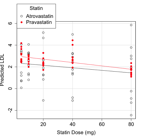
Figure 2. Scatter plot of predicted LDL against dose of a statin drug. Regression lines represent the different statin drugs (Statin1, Statin2).
Question. Based on the graph, can you explain why there will be no statistical differences between levels of the statin drug type, Statin1 (shown open circles) vs. Statin2 (shown closed red circles).
Because we have two predictors (BMI and Statin Dose), you may also elect to use a 3D-scatterplot. Here’s one possible result (Fig. 3).
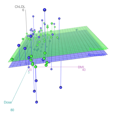
Figure 3. 3D plot of BMI and dose of Statin drugs on change in LDL levels (green Statin2, blue Statin1).
R code for Figure 3.
Graph made in Rcmdr: Graphs → 3D Graph → 3D scatterplot …
scatter3d(ChLDL~BMI+Dose|Statin, data=diabetesCholStatin, fit="linear",
residuals=TRUE, parallel=FALSE, bg="white", axis.scales=TRUE, grid=TRUE,
ellipsoid=FALSE)
Note: Figure 3 is a challenging graphic to interpret. I wouldn’t use it because it doesn’t convey a strong message. With some effort we can see the two planes representing mean differences between the two statin drugs across all predictors, but it’s a stretch. No doubt the graph can be improved by changing colors, for example, but I think the 2d plot Figure 2 works better). Alternatively, if the platform allows, you can use animation options to help your reader see the graph elements. Interactive graphics are very promising and, again, unsurprisingly, there are several R packages available. For this example, plot3d() of the package rgl can be used. Figure 4 is one possible version; I saved images and made animated gif.
Figure 4. An example of a possible interactive 3D plot; the file embedded in this page is not interactive, just an animation.
Diagnostic plots
While visualization concerns are important, let’s return to the statistics. All evaluations of regression equations should involve an inspection of the residuals. Inspection of the residuals allows you to decide if the regression fits the data; if the fit is adequate, you then proceed to evaluate the statistical significance of the coefficients.
The default diagnostic plots (Fig. 5) R provides are available from
Rcmdr: Models → Graphs → Basic diagnostics plots
Four plots are returned
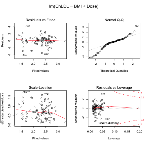
Figure 5. R’s default regression diagnostic plots.
Each of these diagnostic plots in Figure 4 gives you clues about the model fit.
- Plot of residuals vs. fitted helps you identify patterns in the residuals
- Normal Q-Q plot helps you to see if the residuals are approximately normally distributed
- Scale-location plot provides a view of the spread of the residuals
- The residuals vs. leverage plot allows you to identify influential data points.
We introduced these plots in Chapter 17.8 when we discussed fit of simple linear model to data. My conclusion? No obvious trend in residuals, so linear regression is a fit to the data; data not normally distributed Q-Q plot shows S-shape.
Interpreting the diagnostic plots for this problem
The “Normal Q-Q” plot allows us to view our residuals against a normal distribution (the dotted line). Our residuals do no show an ideal distribution: low for the first quartile, about on the line for intermediate values, then high for the 3rd and 4th quartile residuals. If the data were bivariate normal we would see the data fall along a straight line. The “S-shape” suggests log-transformation of the response and or one or more of the predictor variables.
Note that there also seems to be a pattern in residuals vs the predicted (fitted) values. There is a trend of increasing residuals as cholesterol levels increase, which is particularly evident in the “scale-location” plot. Residuals tended to be positive at low and high doses, but negative at intermediate doses. This suggests that the relationship between predictors and cholesterol levels may not be linear, and it demonstrates what statisticians refer to as a monotonic spread of residuals.
The last diagnostic plot looks for individual points that influence, change, or “leverage” the regression — in other words, if a point is removed, does the general pattern change? If so, then the point had “leverage” and thus we need to decide whether or not to include the datum. diagnostic plots Cook’s distance is a measure of the influence of a point in regression. Points with large Cook’s distance values warrant additional checking.
The multicollinearity problem
Statistical model building is a balancing act by the statistician. While simpler models may be easier to interpret and, perhaps, to use, it is a basic truism that the more predictor variables the model includes, the more realistic the statistical model. However, each additional parameter that is added to the statistical model must be independent of all other parameters already in the model. To the extent that this assumption is violated, the problem is termed multicollinearity. If predictor variables are highly correlated, then they are essentially just linear combinations and do not provide independent evidence. For example, one would naturally not include two core body temperature variables in a statistical model on basal metabolic rate, one in degrees Fahrenheit and the other in degrees Celsius, because it is a simple linear conversion between the two units. This would be an example of structural collinearity: the collinearity is because of misspecification of the model variables. In contrast, collinearity among predictor variables may because the data are themselves correlated. For example, if multiple measures of body size are included: weight, height, length of arm, etc., then we would expect these to be correlated, i.e., data multicollinearity.
Collinearity in statistical models may have a number of undesirable effects on a multiple regression model. These include
- estimates of coefficients not stable: with collinearity, values of coefficients depend on other variables in the model; if collinear predictors, then the assumption of independent predictor variables is violated.
- precision of the estimates decreases (standard error of estimates increase).
- statistical power decreases.
- p-values for individual coefficients not trust worthy.
Tolerance and Variance Inflation Factor
Absence of multicollinearity is important assumption of multiple regression. A partial test is to calculate product moment correlations among predictor variables. For example, when we calculate the correlation between BMI and Dose for our model, we get r = 0.101 (P = 0.3186), and therefore would tentatively conclude that there was little correlation between our predictor variables.
A number of diagnostic statistics have been developed to test for multicollinearity. Tolerance for a particular independent variable (Xi) is defined as 1 minus the proportion of variance it shares with the other independent variables in the regression analysis (1 − R2i) (O’Brien 2007). Tolerance reports the proportion of total variance explained by adding the Xi–th predictor variable that is unrelated to the other variables in the model. A small value for tolerance indicates multicollinearity — and that the predictor variable is nearly a perfect combination (linear) of the variables already in the model and therefore should be omitted from the model. Because tolerance is defined in relation to the coefficient of determination you can interpret a tolerance score as the unique variance accounted for by a predictor variable.
A second, related diagnostic of multicollinearity is called the Variance Inflation Factor, VIF. VIF is the inverse of tolerance.

VIF shows how much of the variance of a regression coefficient is increased because of collinearity with the other predictor variables in the model. VIF is easy to interpret: a tolerance of 0.01 has a VIF of 100; a tolerance of 0.1 has a VIF of 10; a tolerance of 0.5 has a VIF of 2, and so on. Thus, small values of tolerance and large values of VIF are taken as evidence of multicollinearity.
Rcmdr: Models → Numerical diagnostics → Variation-inflation factors
vif(RegModel.2)
      BMI     Dose
1.010256 1.010256
A rule of thumb is that if VIF is greater than 5 then there is multicollinearity; with VIF values close to one we would conclude, like our results from the partial correlation estimate above, that there is little evidence for a problem of collinearity between the two predictor variables. They can therefore remain in the model.
Solutions for multicollinearity
If there is substantial multicollinearity then you cannot simply trust the estimates of the coefficients. Assuming that there hasn’t been some kind of coding error on your part, then you may need to find a solution. One solution is to drop one of the predictor variables and redo the regression model. Another option is to run what is called a Principle Components Regression. One takes the predictor variables and runs a Principle Component Analysis to reduce the number of variables, then the regression is run on the PCA components. By definition, the PCA components are independent of each other. Another option is to use ridge regression approach.
Like any diagnostic rule, however, one should not blindly apply a rule of thumb. A VIF of 10 or more may indicate multicollinearity, but it does not necessarily lead to the conclusion that the linear regression model requires that the researcher reduce the number of predictor variables or analyze the problem using a different statistical method to address multicollinearity as the sole criteria of a poor statistical model. Rather, the researcher needs to address all of the other issues about model and parameter estimate stability, including sample size. Unless the collinearity is extreme (like a correlation of 1.0 between predictor variables!), larger sample sizes alone will work in favor of better model stability (by lowering the sample error) (O’Brien 2007).
Questions
- Can you explain why the magnitude of the slope is not the key to statistical significance of a slope? Hint: look at the equation of the t-test for statistical significance of the slope.
- Consider the following scenario. A researcher repeatedly measures his subjects for blood pressure over several weeks, then plots all of the values over time. In all, the data set consists of thousands of readings. He then proceeds to develop a model to explain blood pressure changes over time. What kind of collinearity is present in his data set? Explain your choice.
- We noted that
Dosecould be viewed as categorical variable. ConvertDoseto factor variable (fDose) and redo the linear model. Compare the summary output and discuss the additional coefficients.- Use Rcmdr: Data → Manage variables in active data set → Convert numeric Variables to Factors to create a new factor variable
fDose. It’s ok to use the numbers as factor levels.
- Use Rcmdr: Data → Manage variables in active data set → Convert numeric Variables to Factors to create a new factor variable
- We flagged the change in LDL as likely to be not normally distributed. Create a log10-transformed variable for
ChLDLand perform the multiple regression again.- Write the new statistical model
- Obtain the regression coefficients — are they statistically significant?
- Run basic diagnostic plots and evaluate for
Data set
| ID | Statin | Dose | BMI | LDL | ChLDL |
| 1 | Statin2 | 5 | 19.5 | 3.497 | 2.7147779309 |
| 2 | Statin1 | 20 | 20.2 | 4.268 | 1.2764831106 |
| 3 | Statin2 | 40 | 20.3 | 3.989 | 2.6773769532 |
| 4 | Statin2 | 20 | 20.3 | 3.502 | 2.4306181501 |
| 5 | Statin2 | 80 | 20.4 | 3.766 | 1.7946303961 |
| 6 | Statin2 | 20 | 20.6 | 3.44 | 2.2342950639 |
| 7 | Statin1 | 20 | 20.7 | 3.414 | 2.6353051933 |
| 8 | Statin1 | 10 | 20.8 | 3.222 | 0.8091810801 |
| 9 | Statin1 | 10 | 21.1 | 4.04 | 3.2595985907 |
| 10 | Statin1 | 40 | 21.2 | 4.429 | 1.7639974729 |
| 11 | Statin1 | 5 | 21.2 | 3.528 | 3.3693768458 |
| 12 | Statin1 | 40 | 21.5 | 3.01 | -0.8271542022 |
| 13 | Statin2 | 20 | 21.6 | 3.393 | 2.1117204833 |
| 14 | Statin1 | 10 | 21.7 | 4.512 | 3.1662377996 |
| 15 | Statin1 | 80 | 22 | 5.449 | 3.0083296182 |
| 16 | Statin2 | 10 | 22.2 | 4.03 | 3.0501301624 |
| 17 | Statin2 | 40 | 22.2 | 3.911 | 2.6460344888 |
| 18 | Statin2 | 10 | 22.2 | 3.724 | 2.9456555243 |
| 19 | Statin1 | 5 | 22.2 | 3.238 | 3.2095842825 |
| 20 | Statin2 | 10 | 22.5 | 4.123 | 3.0887629267 |
| 21 | Statin1 | 20 | 22.6 | 3.859 | 5.1525478688 |
| 22 | Statin1 | 10 | 23 | 4.926 | 2.58482964 |
| 23 | Statin2 | 20 | 23 | 3.512 | 2.2919748394 |
| 24 | Statin1 | 5 | 23 | 3.838 | 1.4689995606 |
| 25 | Statin2 | 20 | 23.1 | 3.548 | 2.3407899756 |
| 26 | Statin1 | 5 | 23.1 | 3.424 | 1.2043457967 |
| 27 | Statin1 | 40 | 23.2 | 3.709 | 3.2381790892 |
| 28 | Statin1 | 80 | 23.2 | 4.786 | 2.7486432463 |
| 29 | Statin1 | 20 | 23.3 | 4.103 | 1.2500819426 |
| 30 | Statin1 | 40 | 23.4 | 3.341 | 1.4322916002 |
| 31 | Statin1 | 10 | 23.5 | 3.828 | 1.3817551192 |
| 32 | Statin2 | 10 | 23.8 | 4.02 | 3.0391874265 |
| 33 | Statin1 | 20 | 23.8 | 3.942 | 0.8483284736 |
| 34 | Statin2 | 20 | 23.8 | 2.89 | 1.7211634664 |
| 35 | Statin1 | 80 | 23.9 | 3.326 | 1.9393460444 |
| 36 | Statin1 | 10 | 24.1 | 4.071 | 3.0907410326 |
| 37 | Statin1 | 40 | 24.1 | 4.222 | 1.3223045884 |
| 38 | Statin2 | 10 | 24.1 | 3.44 | 2.472222941 |
| 39 | Statin1 | 5 | 24.2 | 3.507 | 0.0768171794 |
| 40 | Statin2 | 20 | 24.2 | 3.647 | 2.4257575585 |
| 41 | Statin2 | 80 | 24.3 | 3.812 | 1.7105748759 |
| 42 | Statin2 | 40 | 24.3 | 3.305 | 1.9405724055 |
| 43 | Statin2 | 5 | 24.3 | 3.455 | 2.5022137646 |
| 44 | Statin2 | 5 | 24.4 | 4.258 | 3.2280077893 |
| 45 | Statin1 | 5 | 24.4 | 4.16 | 3.4777470262 |
| 46 | Statin2 | 80 | 24.4 | 4.128 | 2.0632471844 |
| 47 | Statin1 | 80 | 24.5 | 4.507 | 3.784421647 |
| 48 | Statin1 | 5 | 24.5 | 3.553 | 0.6957091748 |
| 49 | Statin2 | 10 | 24.5 | 3.616 | 2.6998703189 |
| 50 | Statin2 | 80 | 24.6 | 3.372 | 1.3004010967 |
| 51 | Statin2 | 80 | 24.6 | 3.667 | 1.4181086606 |
| 52 | Statin2 | 5 | 24.7 | 3.854 | 3.1266706892 |
| 53 | Statin1 | 80 | 24.7 | 3.32 | -1.2864388279 |
| 54 | Statin2 | 5 | 24.7 | 3.756 | 2.4236635094 |
| 55 | Statin1 | 40 | 24.8 | 4.398 | 2.907472945 |
| 56 | Statin2 | 40 | 24.9 | 3.621 | 2.3624285593 |
| 57 | Statin1 | 10 | 25 | 3.17 | 1.264656476 |
| 58 | Statin1 | 80 | 25.1 | 3.424 | -2.4369077381 |
| 59 | Statin2 | 10 | 25.1 | 3.196 | 2.0014648648 |
| 60 | Statin2 | 80 | 25.2 | 3.367 | 1.1007041451 |
| 61 | Statin1 | 80 | 25.2 | 3.067 | -0.2315398019 |
| 62 | Statin1 | 20 | 25.3 | 3.678 | 4.6628661348 |
| 63 | Statin2 | 5 | 25.5 | 4.077 | 2.6117051224 |
| 64 | Statin1 | 20 | 25.5 | 3.678 | 2.6330531096 |
| 65 | Statin2 | 5 | 25.6 | 4.994 | 4.1800816149 |
| 66 | Statin1 | 20 | 25.8 | 3.699 | 1.8990314684 |
| 67 | Statin1 | 10 | 25.9 | 3.507 | 4.0637570533 |
| 68 | Statin2 | 20 | 25.9 | 3.445 | 2.3037613081 |
| 69 | Statin1 | 5 | 26 | 4.025 | 2.50142676 |
| 70 | Statin1 | 5 | 26.3 | 3.616 | 0.7408631019 |
| 71 | Statin2 | 40 | 26.4 | 3.937 | 2.5733214297 |
| 72 | Statin2 | 40 | 26.4 | 3.823 | 2.3638394785 |
| 73 | Statin1 | 10 | 26.7 | 4.46 | 2.1741977546 |
| 74 | Statin2 | 5 | 26.7 | 5.03 | 3.845271327 |
| 75 | Statin2 | 10 | 26.7 | 3.73 | 2.7088955103 |
| 76 | Statin2 | 10 | 26.7 | 3.232 | 2.2726268196 |
| 77 | Statin1 | 80 | 26.8 | 3.693 | 1.751169214 |
| 78 | Statin2 | 80 | 27 | 4.108 | 1.8613104992 |
| 79 | Statin2 | 40 | 27.2 | 5.398 | 4.0289773539 |
| 80 | Statin2 | 80 | 27.2 | 4.517 | 2.3489030399 |
| 81 | Statin2 | 20 | 27.3 | 3.901 | 2.7900467077 |
| 82 | Statin1 | 80 | 27.3 | 5.247 | 5.8485450123 |
| 83 | Statin2 | 80 | 27.4 | 3.507 | 1.2478629747 |
| 84 | Statin1 | 20 | 27.4 | 3.807 | -1.0799279924 |
| 85 | Statin2 | 80 | 27.6 | 3.574 | 1.48678931 |
| 86 | Statin1 | 40 | 27.8 | 4.16 | 2.4277532799 |
| 87 | Statin2 | 20 | 28 | 4.501 | 3.2846482963 |
| 88 | Statin2 | 5 | 28.1 | 3.621 | 2.6990067113 |
| 89 | Statin1 | 40 | 28.2 | 3.652 | -1.0912561688 |
| 90 | Statin2 | 40 | 28.2 | 4.191 | 2.8742307203 |
| 91 | Statin2 | 40 | 28.4 | 5.791 | 4.4454535731 |
| 92 | Statin1 | 40 | 28.6 | 4.698 | 3.2028737773 |
| 93 | Statin1 | 5 | 29 | 4.32 | 4.0707532197 |
| 94 | Statin2 | 10 | 29.1 | 3.776 | 2.7512805004 |
| 95 | Statin2 | 5 | 29.2 | 4.703 | 3.6494895215 |
| 96 | Statin2 | 40 | 29.9 | 4.128 | 2.8646910266 |
| 97 | Statin1 | 40 | 30.4 | 4.693 | 4.9837039826 |
| 98 | Statin1 | 20 | 30.4 | 4.123 | 2.2738979752 |
| 99 | Statin1 | 80 | 30.5 | 3.921 | -0.9034376511 |
| 100 | Statin1 | 10 | 36.5 | 4.175 | 3.3114366758 |
Chapter 18 contents
17.8 – Assumptions and model diagnostics for Simple Linear Regression
Introduction
The assumptions for all linear regression:
- Linear model is appropriate.
The data are well described (fit) by a linear model. - Independent values of Y and equal variances.
Although there can be more than one Y for any value of X, the Y‘s cannot be related to each other (that’s what we mean by independent). Since we allow for multiple Y‘s for each X, then we assume that the variances of the range of Y‘s are equal for each X value (this is similar to our ANOVA assumptions for equal variance by groups). Another term for equal variances is homoscedasticity. - Normality.
For each X value there is a normal distribution of Y‘s (think of doing the experiment over and over). - Error
The residuals (error) are normally distributed with a mean of zero.
Note the mnemonic device: Linear, Independent, Normal, Error or LINE.
Each of the four elements will be discussed below in the context of Model Diagnostics. These assumptions apply to how the model fits the data. There are other assumptions that, if violated, imply you should use a different method for estimating the parameters of the model.
Ordinary least squares makes the additional assumption about the quality of the independent variable that e that measurement of X is done without error. Measurement error is a fact of life in science, but the influence of error on regression differs if the error is associated with the dependent or independent variable. Measurement error in the dependent variable increases the dispersion of the residuals but will not affect the estimates of the coefficients; error associated with the independent variables, however, will affect estimates of the slope. In short, error in X leads to biased estimates of the slope.
The equivalent, but less restrictive practical application of this assumption is that the error in X is at least negligible compared to the measurements in the dependent variable.
Multiple regression makes one more assumption, about the relationship between the predictor variables (the X variables). The assumption is that there is no multicollinearity, a subject we will bring up next time (see Chapter 18).
Model diagnostics
We just reviewed how to evaluate the estimates of the coefficients of the model. Now we need to address a deeper meaning — how well the model explains the data. Consider a simple linear regression first. If Ho: b = 0 is not rejected — then the slope of the regression equation is taken to not differ from zero. We would conclude that if repeated samples were drawn from the population, on average, the regression equation would not fit the data well (lots of scatter) and it would not yield useful prediction.
However, recall that we assume that the fit is linear. One assumption we make in regression is that a line can, in fact, be used to describe the relationship between X and Y.
Here are two very different situations where the slope = 0.
Example 1. Linear Slope = 0, No relationship between X and Y
Example 2. Linear Slope = 0, A significant relationship between X and Y
But even if Ho: b = 0 is rejected (and we conclude that a linear relationship between X and Y is present), we still need to be concerned about the fit of the line to the data — the relationship may be more nonlinear than linear, for example. Here are two very different situations where the slope is not equal to 0.
Example 3. Linear Slope > 0, a linear relationship between X and Y
Example 4. Linear Slope > 0, curve-linear relationship between X and Y
How can you tell the difference? There are many regression diagnostic tests, many more than we can cover, but you can start with looking at the coefficient of determination (low R2 means low fit to the line), and we can look at the pattern of residuals plotted against the either the predicted values or the X variables (my favorite). The important points are:
- In linear regression, you fit a model (the slope + intercept) to the data;
- We want the usual hypothesis tests (are the coefficients different from zero?) and
- We need to check to see if the model fits the data well. Just like in our discussions of chi-square, a “perfect fit would mean that the difference between our model and the data would be zero.
Graph options
Using residual plots to diagnose regression equations
Yes, we need to test the coefficients (intercept Ho = 0; slope Ho = 0) of a regression equation, but we also must decide if a regression is an appropriate description of the data. This topic includes the use of diagnostic tests in regression. We address this question chiefly by looking at
- scatterplots of the independent (predictor) variable(s) vs. dependent (response) variable(s).
what patterns appear between X and Y? Do your eyes tell you “Line”? “Curve”? “No relation”? - coefficient of determination
closer to zero than to one? - patterns of residuals plotted against the X variables (other types of residual plots are used to, this is one of my favorites)
Our approach is to utilize graphics along with statistical tests designed to address the assumptions.
One typical choice is to see if there are patterns in the residual values plotted against the predictor variable. If the LINE assumptions hold for your data set, then the residuals should have a mean of zero with scatter about the mean. Deviations from LINE assumptions will show up in residual plots.
Here are examples of POSSIBLE outcomes:
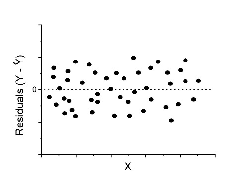
Figure 1. An ideal plot of residuals
Solution: Proceed! Assumptions of linear regression met.
Compare to plots of residuals that differ from the ideal.
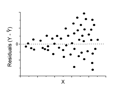
Figure 2. We have a problem. Residual plot shows unequal variance (aka heteroscedasticity).
Solution. Try a transform like the log10-transform.
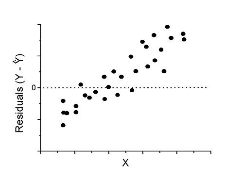
Figure 3. Problem. Residual plot shows systematic trend.
Solution. Linear model a poor fit; May be related to measurement errors for one or more predictor variables. Try adding an additional predictor variable or model the error in your general linear model.
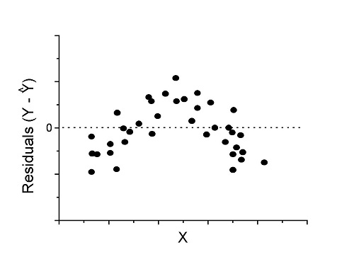
Figure 4. Problem. Residual plot shows nonlinear trend.
Solution. Transform data or use more complex model
This is a good time to mention that in statistical analyses, one often needs to do multiple rounds of analyses, involving description and plots, tests of assumptions, tests of inference. With regression, in particular, we also need to decide if our model (e.g., linear equation) is a good description of the data.
Diagnostic plot examples
Return to our example.Tadpole dataset. To obtain residual plots, Rcmdr: Models → Graphs → Basic diagnostic plots yields four graphs. Graph A is
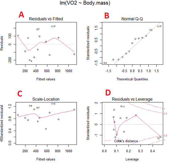
Figure 5. Basic diagnostic plots. A: residual plot; B: Q-Q plot of residuals; C: Scale-location (aka spread-location) plot; D: leverage residual plot.
In brief, we look at plots
A, the residual plot, to see if there are trends in the residuals. We are looking for a spread of points equally above and below the mean of zero. In Figure 5 we count seven points above and six points below zero so there’s no indication of a trend in the residuals vs the fitted VO2 (Y) values.
B, the Q-Q plot is used to see if normality holds. As discussed before, if our data are more or less normally distributed, then points will fall along a straight line in a Q-Q plot.
C, the Scale- or spread-location plot is used to verify equal variances of errors.
D, Leverage plot — looks to see if an outlier has leverage on the fit of the line to the data, i.e., changes the slope. Additionally, provides location of Cook’s distance measure (dashed red lines). Cook’s distance measures the effect on the regression by removing one point at a time and then fitting a line to the data. Points outside the dashed lines have influence.
A note of caution about over-thinking with these plots. R provides a red line to track the points. However, these lines are guides, not judges. We humans are generally good at detecting patterns, but with data visualization, there is the risk of seeing patterns where none exits. In particular, recognizing randomness is not easy. If anything, we may tend to see patterns where none exist, termed apophenia. So yes, by all means look at the graphs, but do so with a plan: red line more or less horizontal? Then no pattern and the regression model is a good fit to the data.
Statistical test options
After building linear models, run statistical diagnostic tests that compliment graphics approaches. Here, simply to introduce the tests, I included the Gosner factor as potential predictor — many of these numerical diagnostics are more appropriate for models with more than one predictor variable, the subject of the next chapter.
Results for the model  were:
were:
lm(formula = VO2 ~ Body.mass + Gosner, data = frogs)

Residuals:
    Min      1Q Median    3Q    Max
-163.12 -125.53 -20.27 83.71 228.56

Coefficients:
           Estimate Std. Error t value  Pr(>|t|)
(Intercept) -595.37     239.87  -2.482 0.03487 *
Body.mass    431.20     115.15   3.745 0.00459 **
Gosner[T.II]  64.96     132.83   0.489 0.63648
---
Signif. codes: 0 '***' 0.001 '**' 0.01 '*' 0.05 '.' 0.1 ' ' 1

Residual standard error: 153.4 on 9 degrees of freedom
  (1 observation deleted due to missingness)
Multiple R-squared: 0.8047, Adjusted R-squared: 0.7613
F-statistic: 18.54 on 2 and 9 DF, p-value: 0.0006432
Question. Note the p-value for the coefficients — do we include a model with both body mass and Gosner Stage? See Chapter 18.5 – Selecting the best model
In R Commander, the diagnostic test options are available via
Rcmdr: Models → Numerical diagnostics
Variance inflation factors (VIF): used to detect multicollinearity among the predictor variables. If correlations are present among the predictor variables, then you can’t rely on the the coefficient estimates — whether predictor A causes change in the response variable depends on whether the correlated B predictor is also included in the model. If correlation between predictor A and B, the statistical effect is increased variance associated with the error of the coefficient estimates. There are VIF for each predictor variable. A VIF of one means there is no correlation between that predictor and the other predictor variables. A VIF of 10 is taken as evidence of serious multicollinearity in the model.
R code:
vif(RegModel.2)
R output
Body.mass Gosner
2.186347 2.186347

round(cov2cor(vcov(RegModel.2)), 3) # Correlations of parameter estimates
         (Intercept) Body.mass Gosner[T.II]
(Intercept)    1.000    -0.958        0.558
Body.mass     -0.958     1.000       -0.737
Gosner[T.II]   0.558    -0.737        1.000
Our interpretation
The output shows a matrix of correlations; the correlation between the two predictor variables in this model was 0.558, large per our discussions in Chapter 16.1 . Not really surprising as older tadpoles (Gosner stage II), are larger tadpoles. We’ll leave the issue of multicollinearity to Chapter 18.1.
Breusch-Pagan test for heteroscedasticity… Recall that heteroscedasticity is another name for unequal variances. This tests pertains to the residuals; we used the scale (spread) location plot (C) above. The test statistic can be calculated as  . The function call is part of the car package, which we download as part of the Rcmdr package. R Commander will pop up a menu of choices for this test. For starters, accept the defaults, enter nothing, and click OK.
R code:
library(zoo, pos=16)
library(lmtest, pos=16)
bptest(VO2 ~ Body.mass + Gosner, varformula = ~ fitted.values(RegModel.2), studentize=FALSE, data=frogs)
R output
Breusch-Pagan test

data:  VO2 ~ Body.mass + Gosner
BP = 0.0040766, df = 1, p-value = 0.9491
Our interpretation
A p-value less than 5% would be interpreted as statistically significant unequal variances among the residuals.
Durbin-Watson for autocorrelation… used to detect serial (auto)correlation among the residuals, specifically, adjacent residuals. Substantial autocorrelation can mean Type I error for one or more model coefficients. The test returns a test statistic that ranges from 0 to 4. A value at midpoint (2) suggests no autocorrelation. Default test for autocorrelation is r > 0.
R code:
dwtest(VO2 ~ Body.mass + Gosner, alternative="greater", data=frogs)
R output
Durbin-Watson test

data:  VO2 ~ Body.mass + Gosner
DW = 2.1336, p-value = 0.4657
alternative hypothesis: true autocorrelation is greater than 0
Our interpretation
The DW statistic was about 2. Per our definition, we conclude no correlations among the residuals.
RESET test for nonlinearity… The Ramsey Regression Equation Specification Error Test is used to interpret whether or not the equation is properly specified. The idea is that fit of the equation is compared against alternative equations that account for possible nonlinear dependencies among predictor and dependent variables. The test statistic follows an F distribution.
R code:
resettest(VO2 ~ Body.mass + Gosner, power=2:3, type="regressor", data=frogs)
R output
RESET test

data:  VO2 ~ Body.mass + Gosner
RESET = 0.93401, df1 = 2, df2 = 7, p-value = 0.437
Our interpretation
Also a nonsignificant test — adding a power term to account for a nonlinear trend gained no model fit benefits, p-value much greater than 5%.
Bonferroni outlier test. Reports the Bonferroni p-values for testing each observation to see if it can be considered to be a mean-shift outlier (a method for identifying potential outlier values — each value is in turn replaced with the mean of its nearest neighbors, Lehhman et al 2020). Compare to results of VIF. The objective of outlier and VIF tests is to verify that the regression model is stable, insensitive to potential leverage (outlier) values.
R code:
outlierTest(LinearModel.3)
R output
No Studentized residuals with Bonferroni p < 0.05
Largest |rstudent|:
  rstudent unadjusted p-value Bonferroni p
7 1.958858        0.085809              NA
Our interpretation
ccc
Response transformation… The concept of transformations of data to improve adherence to statistical assumptions was introduced in Chapters 3.2, 13.1, and 15.
R code:
> summary(powerTransform(LinearModel.3, family=”bcPower”))
R output
bcPower Transformation to Normality
    Est Power Rounded Pwr Wald Lwr Bnd Wald Upr Bnd
Y1     0.9987           1       0.2755       1.7218

Likelihood ratio test that transformation parameter is equal to 0
   (log transformation)
                           LRT df      pval
LR test, lambda = (0) 7.374316  1 0.0066162

Likelihood ratio test that no transformation is needed
                                LRT df    pval
LR test, lambda = (1) 0.00001289284  1 0.99714
Our interpretation
ccc
Questions
- Referring to Figures 1 – 4 on this page, which plot best suggests a regression line fits the data?
- Return to the electoral college data set and your linear models of Electoral vs. POP_2010 and POP_2019. Obtain the four basic diagnostic plots and comment on the fit of the regression line to the electoral college data.
- residual plot
- Q-Q plot
- Scale-location plot
- Leverage plot
- With respect to your answers in question 2, how well does the electoral college system reflect the principle of one person one vote?
Chapter 17 contents
- Introduction
- Simple Linear Regression
- Relationship between the slope and the correlation
- Estimation of linear regression coefficients
- OLS, RMA, and smoothing functions
- Testing regression coefficients
- Regression model fit
- Assumptions and model diagnostics for Simple Linear Regression
- References and suggested readings (Ch17 & 18)