6.4 – Types of probability
Introduction
By probability, we mean a number that quantifies the uncertainty associated with a particular event or outcome. If an outcome is certain to occur, the probability is equal to 1; if an outcome cannot happen, the probability is equal to zero. Most events we talk about in biology have probability somewhere in between.
A basic understanding, or at least an appreciation for probability is important to your education in biostatistics. Simply put, there is no certainty in biology beyond simple expectations like Benjamin Franklin’s famous quip about “death and taxes…”
Discrete probability
You are probably already familiar with discrete probability. For example, what is the probability that a single toss of a fair coin will result in a “heads?” The outcomes of the coin toss are discrete, categorical, either “heads” or “tails.”
Note. Obviously, this statement assumes a few things — coin tossed not in a vacuum, although possible, we ignore possibility of
And for ten tosses of the coin? And more cogently, what is the probability that you will toss a coin ten times and get all ten “heads?” While different in tone, these are discrete outcomes. An important concept is independence. Are the multiple events independent? In other words, does the toss of coin on the first attempt affect the toss of the coin on the second attempt and so on up to the tenth toss? At least in principle the repeated tosses are independent so to find the probability you just multiply each event’s probability to get the total. In contrast, if one or more events are not independent but somehow influence the behavior of the next event, then you add the probabilities for each dependent event. We can do better than simply multiply or add events one at a time; depending on the number of discrete outcomes it is very likely that someone has already calculated all possible outcomes and come up with an equation. In the case of the tossing of two coins this is a binomial equation problem and repeat tosses can be modeled by use of the Bernoulli distribution.
Now, try this on for size. What is the probability that the next child born at Kapiolani Medical Center in Honolulu will be assigned female?
We just described a discrete random variable, which can only take on discrete or “countable” numbers. This distribution of values is the probability mass function. The probability of a one fatal airline accident in a year exactly on 20.1 is practically zero (the area under a point along the curve is zero), so we can get the probability of a range of values around the point as our answer.
Continuous probability
Many events in biology are of degree, not kind. It is kind of awkward to think about it, but for a sample of adult house mice drawn from a population, what is the probability of obtaining a mouse that is 20.0000 grams (g) in weight? Each possible value of body mass for a mouse is considered an event, just like in our example of tossing a coin. But clearly, we don’t expect to get a lot of mice that are exactly 20.0000 g in weight. For variables like body mass, the type of data we collect is continuous, and the probability values need to be rethought along a continuum of possible values and, in turn, how likely each value is for a mouse. Although it is theoretically possible that a mouse could weigh ten pounds, we know by experience that this is impossible. Adult mice weigh between 15 and 50 g or there about.
We just described a continuous random variable, which can take on any value between a specific interval of values. This distribution of values is the probability density function. The probability of a mouse’s weight falling exactly on 20.1 is practically zero (the area under a point along the curve is zero), so we can get the probability of a range of values around the point as our answer.
In statistical inference, following our measurements of the variables from our sample drawn from a population, we make conclusions with the following kind of caveat: “the mean body mass for this strain of mouse is 20 g.” That is our best estimate of the mean (middle) for the population of mice, more specifically, for the body mass of the mice. Here, the variable body mass is more formally termed a random variable. This implies that there is in fact a true population mean body mass for the mice and that any deviations from that mean are due to chance. In statistics we don’t settle for a single point estimate of the population mean. You will find most reporting of estimates of random variables is accompanies by a statement like, the mean was 20g with a 95% probability that the true population mean is between 18.9 and 21 g. This is called the 95% confidence interval for the mean and it takes into account how good of an estimate our sample is likely to be relative to the true population value. Not only are we saying that we think the population mean is 20g, but we’re willing to say that we are 95% certain that the true value must be between a lower limit (18.9 g) and and upper limit (21 g). In order to make this kind of statement we have to assume a distribution that will describe the probability of mouse weights. For many reasons we usually assume a normal distribution. Once we make this assumption we can calculate how probable a particular weight is for a mouse.
We introduced how to calculate Confidence Intervals in Chapter 3.4 and will extend this in Chapters .
Types of probability
To begin refining our concept of probability, it is sometimes useful to distinguish among kinds of probabilities:
- between theoretical and empirical;
- between subjective and objective.
In most cases, including your statistics book, we would begin our discussion of probability by talking of some probabilities for events we’re familiar with.
- The theoretical probability of heads appearing the next time you flip a fair coin is 1/2 or 50%. As long as we’re talking about a fair coin, the probability of a heads appearing each time you flip the coin remains 50%. We can check this by conducting and experiment: out of 10 tosses, how many heads appear? The answer would be an empirical probability, and we understand the chance in an objective manner (no interpretation needed).
- The theoretical probability that a “5” will appear on the face of a fair dice after a toss is 1/6 or 16.667%. Again, as long as we’re talking about a fair dice, the probability of a “5” appearing each time you roll the dice remains 16.667%.
- The probability that at birth, a human baby’s sex will be male about 1/2 or 50%. This is an empirical probability based on millions of observations. Changes in technology, and ethical standards notwithstanding, the probability will remain the same.
- The probability of the birth of a Downs syndrome baby is 1/800, but increases with age until by age 45, the chance is 1/12. Again, these are empirical and objective.
- The probability of winning the Publisher’s Clearing House Sweepstakes is about 1 in 100 million. This probability is theoretical, it is also objective; however, by adding lots of twists to the game, by having multiple opportunities and by giving the appearance that a person must purchase a magazine, some players perceive their chances as increasing or decreasing by their efforts (=subjective).
R and distributions
R Commander: Distributions menus give four options
- Quantiles
- Probabilities
- Plot
- Sampling
Questions
1. Define and distinguish, with examples
- discrete and continuous probability
- theoretical and empirical probability
- subjective and objective probability
Chapter 6 contents
- Introduction
- Some preliminaries
- Ratios and proportions
- Combinations and permutations
- Types of probability
- Discrete probability distributions
- Continuous distributions
- Normal distribution and the normal deviate
- Moments
- Chi-square distribution
- t distribution
- F distribution
- References and suggested readings
6.1 – Some preliminaries
Introduction
OK, you say, I get it: statistics is important, and if I am to go on as a biologist, I should learn some biostatistics. Let’s get on with it, start with the equations and the problems already!
Before we review probability theory and introduce risk analysis I want to spend some time to emphasize that at issue is critical thinking, so please bear with me (Fig. 1).
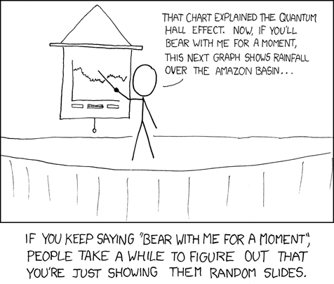
Figure 1. https://xkcd.com/365/
How likely?
As we start our journey in earnest, we start with the foundations of statistics, probability. Probability is something we measure, or estimate, about whether something, an event, will occur. We speak about how likely an event is to occur, and this is quantified by the probability. Probabilities are given a value between 0 and 1: at 0% chance, the event will not happen; 100% chance, the event is certain to happen.
If probability is the chance that an event will occur, then risk is the probability of an event occurring over a specified period of time. I introduce our discussion of probability through a risk analysis. I like to start this discussion by relaying something I overheard, while we were all standing on a lava field on the slopes of Kilauea back in November of 1998 (Kilauea erupted with lava flow more or less continually between 1983 and 2018; 5 Jan 2023, started up again).

Figure 2. View of Kamokuna Lava Bench, eruption of Pu`u `O`o, Kilauea, November 1998. Photo by S. Dohm.
The Volcanoes National Park hadn’t established barricades at the end of Chain of Craters Road, and people were walking to see new lava flows. The night we went, we met a park ranger who announced to us that the Park Service believed it was unsafe for us to walk out to see new lava flows because the area was unstable. Someone (not in my group), snapped back, “Oh, what are the chances that that will happen?” Of course, the ranger couldn’t quote a chance between zero and 100% for that particular evening. The ranger was saying the risk had increased, based on their subjective, but experienced opinion.
As you can see in Figure 2, we went anyway. I have been thinking about her question ever since. We were lucky — some of the same area collapsed two weeks later (SOEST information, eruption about episode 55).
Cool picture though.
Multiple events
I have two coins, a dime and a quarter, in my pocket; when I place the coins on the table, what are the chances that both coins will show heads? A blood sample from a crime scene was typed for two Combined DNA Index System (CODIS) Short Tandem Repeat (STR) loci, THO1 (allele 9.3) and TPOX (allele 8), the same allele types for the defendant. What are the chances of a random match, someone other than the defendant has the same genetic profile? For two or more independent events we can get the answers by using the product rule.

The two coins are independent, therefore the chance that both are placed heads up is 25% — we would expect to see this combined event one out of every four times. This is an illustration of the counting rule, aka fundamental counting principle: if there are n ways to do one thing (n elements in set A), and m ways to do another thing (m elements in set B), then there are  ways to do both things (combination of elements of A and B sets).
For the DNA profile CODIS problem (cf. Chapter 4, National Research Council 1996), the two alleles are both the most common observed in US Caucasian population at 30.45% and 54.7%, respectively (Moretti et al 2016). Assuming the individual was homozygous at both loci (i.e., THO19.3,9.3 and TPOX8,8), then the genotype frequencies (p2) are:


Since THO1 is located on the p arm of chromosome 11, and TPOX is on the p arm of chromosome 2, the two loci are independent and therefore should be in linkage disequilibrium. We can use the product rule to get the probability of the DNA profile for the sample, 2.8%

If two events are not independent, then the product rule cannot be used. For example, CODIS STR D5S818 and CSF1PO are both located on the q arm of chromosome 5 and are therefore linked and not independent (the recombination frequency is about 0.25). The common allele for D5S818 is 11 at 40.84% and for CSF1PO the allele is 12 at 34.16%. Thus the chance that the two most common alleles is not simply the product rule result of 14%, instead we need to view this problem as one of dependent events.
Kinds of probability
So, how does one go about estimating the likelihood that a particular event, whether it is collapse of a lava delta, or that a person will have a heart attack? The probability of lava delta collapse or of heart attack are examples of empirical probability, as opposed to a theoretical probability. Despite many years of effort, we have no applicable theory that we can apply to say, if a person does this, and that, then a heart attack will happen. But we do have a body of work documenting how often heart attacks occur, and when they occur in association with certain risk factors. Similarly, progress is being made to determine markers of risk of lava field collapse (Di Traglia et al. 2018). Analogously, this is the essential goal of risk analysis in epidemiology. We know of associations between cholesterol and heart attack risk, for example, but we also know that high cholesterol does not raise the probability of the event (heart attack) to 100%. How is this uncertainty part of statistics? Or perhaps you are a molecular scientist in training and have learned about how to assess results of a Western blot where typically the results are scored as “yes” or “no.” How is this relevant to statistics and probability?
A misconception about statistics and statistical thinking
There’s a long history of skepticism of conclusions from health studies, in part because it seems the advice flips. For example,
- Coffee is bad for you (Medical News Today January 2008)
- Coffee is good for you (NBC News July 2018)
- Even light drinking can be harmful to health (Science Daily, January 2022)
- Seven science-backed reasons beer is good for you (NBC News August 2017)
- Meat and cheese may be as bad for you as smoking (Science Daily, March 2014)
- Cheese actually isn’t bad for you (WIRED, February 2021)
The common thread is these studies are assessment of risk: about studies that seem to conclude “only: with statements of probability.
Perhaps you may have heard …? “There are lies and then there is statistics“. The full quote reads as follows:
Figures often beguile me, particularly when I have the arranging of them myself; in which case the remark attributed to Disraeli would often apply with justice and force: “There are three kinds of lies: lies, damned lies and statistics.” – Autobiography of Mark Twain (www.twainquotes.com/Lies.html).

Figure 3. Mark Twain. Image from The Miriam and Ira D. Wallach Division of Art, Prints and Photographs: Photography Collection, The New York Public Library. “Mark Twain in Middle Life” The New York Public Library Digital Collections. 1860 – 1920. https://digitalcollections.nypl.org/items/510d47d9-baec-a3d9-e040-e00a18064a99
Twain attributed the remarks to Benjamin Disraeli, the prime minister of Britain during much of Queen Victoria’s reign, but others have not been able to document this utterance to that effect. Still others believe that the “3-lies” quote belongs to Leonard Courtney, an English mathematician and statistician (1847-1929) (see University of York web site for more).
What is meant by this quote? Tossing aside cynicism — or healthy skepticism of authority one should have, whether that authority is a scientist or a politician(within reason, please!) — what this quote means is that it seems that results of very similar studies are in conflict. To some, this is part of the replication crisis in science (Baker 2016). There’s a perception that one can say just about anything with a number. Partly this is a matter of semantics, but also there is legitimacy to this concern. However, it is not necessarily the case that statistics have been intentionally done to mislead, rather, there is evidence that researchers are not always using proper statistical procedures.
One word, several meanings
We use the term statistics in multiple ways, all correct, but not all equal. For example, a statistic may refer to a number used to describe a population characteristic. From the 2010 U.S. census, we learn that the racial (self-reported) make-up of the U.S. population (then at 303 million) was 72.4% “white” and 12.6% “black” self-reported. In this sense, a statistic is something you calculate as a description. Do you recall the distinction between “statistic” and “statistics” discussed in Chapter 2?
Secondly, two studies essentially about the same topic, yet reaching seemingly different conclusions, may differ in the assumptions employed. It should be obvious that if different assumptions are used, researchers may reach different outcomes.
Finally, how we communicate statistics can be misleading. For example, use of percentages in particular can be confusing, especially in communication of the chance that some event may happen to us (e.g., incidence of disease: number of new cases in a specific time period, compared to prevalence of a disease: number of cases of a disease in a specific period of time). On the one hand, percentages seem easy. A percentage is simply a proportion multiplied by 100%, and takes any value between 0% and 100%.
When a product says that it kills 99.99% of all germs on contact, do you feel better? Here’s a cartoon to consider as you think about that statement.
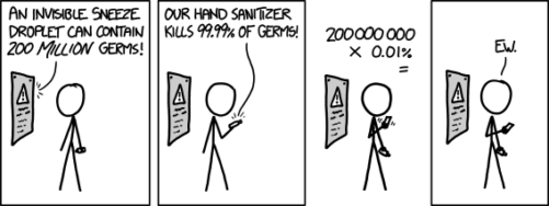
Figure 3. xkcd comic strip, from https://imgs.xkcd.com/comics/hand_sanitizer.png
Of course numbers cannot be used to justify simultaneously mutually exclusive conclusions, but being able to recognize careless (or deliberate) miscommunication with numbers, well, this needs to be part of your skill set. Here’s a little exercise from transportation safety to ponder as you reflect on the subject of lies and statistics. rather, as you read this next section I ask that you consider
- are the correct statistical descriptors in use?
- what assumptions are being made?
- does the reporting of percentages lead to clear conclusions?
Some concluding thoughts about “lies and statistics”
Statistics is tricky because there are assumptions to be made. And you have to be clear in your thinking.
If the assumptions hold true, then we aren’t lying, and Twain had it wrong.
But if we disagree on the assumptions, then we will necessarily have to disagree on the conclusions drawn from the calculated numbers (the statistics). Risk analysis in particular, but statistics in general, is a tricky business because many assumptions need to be made, and we won’t necessarily have all of the relevant information available to make sure our assumptions are truthful. But it is the assumptions that matter: if we agree with the assumptions that are made, then we have confidence in the conclusions drawn from the statistics.
In a typical statistics course, we would spend a bunch of time on probability. We will here as well, but in the context of risk analysis and in the other contexts, in a less than formal presentation on the subject of probability. For example, in talking about inference, the testing of null hypotheses and estimating the probability that the null hypothesis is correct, I will say things like, “Imagine we repeated the experiment a million times — how many times by chance would we think a correct null hypothesis would none the less be rejected?”
There’s no real substitute for a formal course in probability theory and you should be aware that this foundation is pretty important if you go forward with biostatistics and epidemiology. For now, I will simply refer you to chapters 1, 2 and 3 of a really nice online book on probability from one of the masters, Richard Jeffrey (1926 – 2002; click here to go to Wikipedia). Much of what I will present to you follows from similar discussions.
My aim is to teach you what you need about probability theory by the doing. In the next couple of days we will deal with an aspect of risk analysis, namely a consideration of CONDITIONAL PROBABILITY and Baye’s Theorem that will help you evaluate claims such as the one made for airline safety. Risk analysis is tricky, but it is not a subject above and beyond our abilities; by applying some of the rules of statistical reasoning, we can check claims based on statistics. A healthy degree of skepticism is part of becoming a scientist. Do try this at home!
Some examples to consider: what is the relative risk for the following scenarios?
1. Drug testing at the workplace: risk of a worker, who does not use illegal drugs, registering positive (false positives in drug testing);
2. Positive HIV from blood sample from USA male with no associated risks (e.g., intravenous drug user), false positives in HIV testing; false positives with mammography;
3. Benefits versus risks of taking a statin drug (drug that reduces serum cholesterol levels) to a person with no history of heart disease.
4. Is it safer to travel by car or by airliner? We’ll break this problem down in the next section.
What we are looking for is the probability of an occurrence of a particular event: that a person who does not use illegal drugs may nonetheless test positive; we are looking for a way to make rational decisions and understanding probability is the foundation.
Questions
- What do you make of the claim (joke) that “There are lies and then there are statistics?”
- For the various proportions listed, can these also be considered to be rates?
- Distinguish between empirical and theoretical probability; use examples.
- CODIS STR D5S818 and CSF1PO are both located on the q arm of chromosome 5 and are therefore linked and not independent (the recombination frequency is about 0.25). The common allele for D5S818 is 11 at 40.84% and for CSF1PO the allele is 12 at 34.16%. Given that the person has allele 11 at D5S818 (genotype 11,11), what are the chances that they also have allele 12 at CSF1PO (genotype 12,12)?
Chapter 6 contents
- Introduction
- Some preliminaries
- Ratios and proportions
- Combinations and permutations
- Types of probability
- Discrete probability distributions
- Continuous distributions
- Normal distribution and the normal deviate (Z)
- Moments
- Chi-square distribution
- t distribution
- F distribution
- References and suggested readings
6 – Probability, Distributions
Introduction
Probability is how likely something, an event, is likely to occur. Thus, an important concept to appreciate is that in many cases, like R.A. Fisher’s Lady tasting tea analogy, we can count in advance all possible outcomes of an experiment. On the other hand, for many more experiments, we cannot count all possible outcomes of the sample space, either because they are too numerous or simply unknowable. In such cases, applying theoretical probability distributions allow us to circumvent the countability problem. Whereas empirical probability distributions are frequency counts of observations, theoretical probabilities are based on mathematical formulas.
Much of classical inferential statistics, especially the kind one finds in introductory courses like ours, are built on probability distributions. ANOVA, t-tests, linear regression, etc., are parametric tests and assume errors are distributed according to a particular type of distribution, the normal or Gaussian distribution.
A probability distribution is a list of probabilities for each possible outcome of a discrete random variable in an entire population. Depending on the data type, there are many classes of probability distributions. In contrast, probability density functions are used to for continuous random variables. This chapter begins with basics of probability then gently introduces probability distributions. In the other sections of this chapter we describe several probability density functions. Emphasis is placed on the normal distribution, which underlies most parametric statistics.
Chapter 6 contents
- Introduction
- Some preliminaries
- Ratios and proportions
- Combinations and permutations
- Types of probability
- Discrete probability distributions
- Continuous distributions
- Normal distribution and the normal deviate (Z)
- Moments
- Chi-square distribution
- t distribution
- The F distribution
- References and suggested readings