12.2 – One way ANOVA
Introduction
In ANalysis Of VAriance, or ANOVA for short, we likewise have tools to test the null hypothesis of no difference between between categorical independent variables — often called factors when there’s just a few levels to keep track of — and a single, dependent response variable. But now, the response variable is quantitative, not qualitative like the  tests.
Analysis of variance, ANOVA, is such an important statistical test in biology that we will take the time to “build it” from scratch. We begin by reminding you of where you’ve been with the material.
We already saw an example of this null hypothesis. When there’s only one factor (but with two or more levels), we call the analysis of means and “one-way ANOVA.” In the independent sample t-test, we tested whether two groups had the same mean. We made the connection between the confidence interval of the difference between the sample means and whether or not it includes zero (i.e., no difference between the means). In ANOVA, we extend this idea to a test of whether two or more groups have the same mean. In fact, if you perform an ANOVA on only two groups, you will get the exact same answer as the independent two-sample t-test, although they use different distributions of critical values (t for the t-test, F for the ANOVA — a nice little fact for you square the t-test statistic, you’ll get the F-test statistic:  ).
).
Let’s say we have an experiment where we’ve looked at the effect of different three different calorie levels on weight change in middle-aged men.
I’ve created a simulated dataset which we will use in our ANOVA discussions. The data set is available at the end of this page (scroll down or click here).
We might graph the mean weight changes ( SEM); Below are two possible outcomes of our experiment (Fig. 1).
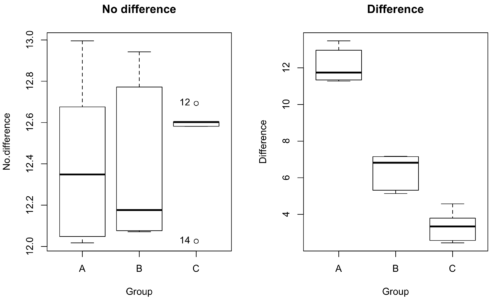
Figure 1. Hypothetical results of an experiment, box plots. Left, no difference among groups; Right, large differences among groups.
As statisticians and scientists, we would first calculate an overall or grand mean for the entire sample of observations; we know this as the sample mean whose symbol is  . But this overall mean is made up of the average of the sample means. If the null hypothesis is true, then the all of the sample means all estimate the overall mean. Put another way, being a member of a treatment group doesn’t matter, i.e., there is no systematic effect, all differences among subjects are due to random chance.

The hypotheses among are three groups or treatment levels then are:

Null that there are no differences among the group means. And the alternative hypotheses include any (or all) of the following possibilities

or maybe

or… have we covered all possible alternate outcomes among three groups?
In either case, we could use one-way ANOVA to test for “statistically significant differences.”
Three important terms you’ll need for one-way ANOVA
FACTOR: We have one factor of interest. For example, a factor of interest might be
- Diet fed to hypertensive subjects (men and women)
- Distribution of coral reef sea cucumber species in archipelagos
- Antibiotic drug therapy for adolescents with Acne vulgaris (click see Webster 2002 for review).
Note 1: Character vs factor. In R programming, while it is true that a treatment variable can be a character vector like Gender*, such vectors are handled by R as string. In contrast, by claiming Gender as a factor, R handles the variable as a nominal data type. Hence, ANOVA and other GLM functions expect any treatment variable to be declared as a factor:
Gender <- c("Gender non-conforming", "Men", "Non-binary", "Transgender", "Women", "Declined"); Gender
[1] "Gender non-conforming" "Men" "Non-binary" "Transgender"
[5] "Women" "Declined"
# it’s a string vector, not a factor
is.factor(Gender)
[1] FALSE
Change string vector to a factor.
Gender <- as.factor(Gender); is.factor(Gender) [1] TRUE
* For discussions of ethics of language inclusivity and whether or not such information should be gathered, see Henrickson et al 2020.
LEVELS: We can have multiple levels (2 or more) within the single factor. Some examples of levels for the Factors listed:
- Three diets (DASH), diet rich in fruits & vegetables, control diet)
- Five archipelagos (Hawaiian Islands, Line Islands, Marshal Islands, Bonin Islands, and Ryukyu Islands)
- Five antibiotics (ciprofloxacin, cotrimoxazole, erythromycin, doxycycline, minocycline).
RESPONSE: There is one outcome or measurement variable. This variable must be quantitative (i.e., on the ratio or interval scale). Continuing our examples then
- Reduction in systolic pressure
- Numbers of individual sea cucumbers in a plot
- number of microcomedo.
Note 2: A comedo is a clogged pore in the skin; a microcomedo refers to the small plug. Yes, I had to look that up, too.
The response variable can be just about anything we can measure, but because ANOVA is a parametric test, the response variable must be normally distributed!
Note on experimental design
As we discuss ANOVA, keep in mind we are talking about analyzing results from an experiment. Understanding statistics, and in particular ANOVA, informs how to plan an experiment. The basic experimental design is called a completely randomized experimental design, or CDR, where treatments are assigned to experimental units at random.
In this experimental design, subjects (experimental units) must be randomly assigned to each of these levels of the factor. That is, each individual should have had the same probability of being found in any one of the levels of the factor. The design is complete because randomization is conducted for all levels, all factors.
Thinking about how you would describe an experiment with three levels of some treatment, we would have
Table 1. Summary statistics of three levels for some ratio scale response variable.
| Level 1 |
sample mean1 |
sample standard deviation1 |
| Level 2 |
sample mean2 |
sample standard deviation2 |
| Level 3 |
sample mean3 |
sample standard deviation3 |


Note 3: Table 1 is the basis for creating the box plots in Figure 1.
ANOVA sources of variation
ANOVA works by partitioning total variability about the means (the grand mean, the group means). We will discuss the multiple samples and how the ANOVA works in terms of the sources of variation. There are two “sources” of variation that can occur:
- Within Group Variation
- Among Groups Variation
So let’s look first at the variability within groups, also called the Within Group Variation.
Consider and experiment to see if DASH diet reduces systolic blood pressure in USA middle-aged men and women with hypertension (Moore et al 2001). After eight weeks we have
We get the corrected sum of squares, SS, for within group
![\begin{align*} within-groups \ SS = \sum_{i=1}^{k}\left [ \sum_{j=1}^{n_{i}}\left ( X_{ij}-\bar{X}_{i} \right )^2 \right ] \end{align*}](https://biostatistics.letgen.org/wp-content/ql-cache/quicklatex.com-f4b56281eaa75640199e7db56cb40586_l3.png "Rendered by QuickLaTeX.com")
and the degrees of freedom, DF, for within groups

where i is the identity of the groups,  is the individual observations within group i,
  is the group i mean, ni is the sample size within each group, N is the total sample size of all subjects for all groups, and k is the number of groups.
Importantly, this value is also referred to as “error sums of squares” in ANOVA. It’s importance is as follows — In our example, the within group variability would be zero if and only if all subjects within the same diet lost exactly the same amount of weight. This is hardly ever the case of course in a real experiment. Because there are almost always some other unknown factors or measurement error that affect the response variable, there will be some unknown variation among individuals who received the same treatment (within the same group). Thus, the error variance will generally be larger than zero.
The first point to consider: your ANOVA will never result in statistical differences among the groups if the error variance is greater than the second type of variability, the variability between groups.
The second type of variability in ANOVA is that due to the groups or treatments. Individuals given a calorie-restricted diet will loose some weight; individuals allowed to eat a calorie-rich diet likely will gain weight, therefore there will be variability (a difference) due to the treatment. So we can calculate the variability among groups. We get the corrected sum of squares for among groups

and the degrees of freedom for among groups

where i is the identity of the groups, is the grand mean as defined in Measures of Central Tendency (Chapter 3.1), is the group i mean, ni is the sample size within each group, N is the total sample size of all subjects for all groups, and k is the number of groups.
The sums of squares here is simply subtracting the mean of each population from the overall mean.
- If the Factor is not important in explaining the variation among individuals then all the population means will be similar and the sums of squares among populations would be small.
- If the Factor is important in explaining some of the variation among the individuals then all the population means will NOT be the same and the sums of squares among populations would be large.
Finally, we can identify the total variation in the entire experiment. We have the total sum of squares.

Thus, the insight of ANOVA is that variation in the dataset may be attributed to a portion explained by differences among the groups and differences among individual observations within each group. The inference comes from recognizing that if the among group effect is greater than the within group effect, then there will be a difference due to the treatment levels.
Mean squares
To decide whether the variation associated with the among group differences are greater than the within group variation, we calculate ratios of the sums of squares. These are called Mean Squares or MS for short. The ratio of the Mean Squares is called F, the test statistic for ANOVA.
For the one-way ANOVA we will have two Mean Squares and one F, tested with degrees of freedom for both the numerator  , and denominator
  ).
).
The Mean Square for (among) groups is

The Mean Square for error is

And finally, the value for F, the test statistic for ANOVA, is

Worked example with R
A factor with three levels, A, B, and C
group <- c("A", "A", "A", "B", "B", "B", "C", "C", "C")
and their responses, simulated
response <- c(10.8, 11.8, 12.8, 6.5, 7, 8, 3.8, 2.8, 3)
We create a data frame
all <- data.frame(group, response)
Of course, you could place the data into a worksheet and then import the worksheet into R. Regardless, we now have our dataset.
Now, call the ANOVA function, aov, and assign the results to an object (e.g., Model.1)
Model.1 <- aov(response ~ group, data=all)
Now, visualize the ANOVA table
summary(Model.1)
and the output from R, the ANOVA table, is shown below
Note 4: Rcmdr: Statistics → Means → One-way ANOVA… see figures 2 and 3 below
Table 2. Output from aov() command, the ANOVA table, for the “Difference” outcome variable.
           Df   Sum Sq    Mean Sq   F value       Pr(>F)
group       2   111.16      55.58     89.49    0.0000341 ***
Residuals   6     3.73       0.62
---
Signif. codes: 0 '***' 0.001 '**' 0.01 '*' 0.05 '.' 0.1 ' ' 1
Let’s take the ANOVA table one row at a time
- The first row has subject headers defining the columns.
- The second row of the table “groups” contains statistics due to group, and provides the comparisons among groups.
- The third row, “Residuals” is the error, or the differences within groups.
Moving across the columns, then, for each row, we have in turn,
- the degrees of freedom (there were 3 groups, therefore 2 DF for group),
- the Sums of Squares, the Mean Squares,
- the value of F, and finally,
- the P-value.
R provides a helpful guide on the last line of the ANOVA summary table, the “Signif[icance] codes,” which highlights the magnitude of the P-value.
What to report? ANOVA problems can be much more complicated than the simple one-way ANOVA introduced here. For complex ANOVA problems, report the ANOVA table itself! But for the one-way ANOVA it would be sufficient to report the test statistic, the degrees of freedom, and the p-value, as we have in previous chapters (e.g., t-test, chi-square, etc.). Thus, we would report:
F = 89.49, df = 2 and 6, p = 0.0000341
where F = 89.49 is the test statistic, df = 2 (degrees of freedom for the among group mean square) and 6 (degrees of freedom for the within group mean square), and p = 0.0000341 is the p-value.
In Rcmdr, the appropriate command for the one-way ANOVA is simply
Rcmdr: Statistics → Means
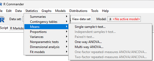
Figure 2. Screenshot Rcmdr select one-way ANOVA
which brings up a simple dialog. R Commander anticipates factor (Groups) and Response variable. Optional, choose Pairwise comparisons of means for post-hoc test (Tukey’s) and, if you do not want to assume equal variances (see Chapter 13), select Welch F-test.

Figure 3. Screenshot Rcmdr select one-way ANOVA options.
Questions
1. Review the example ANOVA Table and confirm the following
- How many levels of the treatment were there?
- How many sampling units were there?
- Confirm the calculation of
 and using the formulas contained in the text.
 - Confirm the calculation of F using the formula contained in the text.
- The degrees of freedom for the F statistic in this example were 2 and 6 (F2,6). Assuming a two-tailed test with Type I error rate of 5%, What is the critical value of the F distribution (see Appendix 20.4)
2. Repeat the one-way ANOVA using the simulated data, but this time, calculate the ANOVA problem for the “No.difference” response variable.
3. Leaf lengths from three strains of Arabidopsis thaliana plants grown in common garden are shown in Fig. 2. Data are provided for you in the following R script.
arabid <- c("wt","wt","wt","AS1","AS1","AS1","AS2","AS2","AS2")
leaf <- c(4.909,5.736,5.108,6.956,5.809,6.888,4.768,4.209,4.065)
leaves <- data.frame(arabid,leaf)
- Write out a null and alternative hypotheses
- Conduct a test of the null hypothesis by one-way ANOVA
- Report the value of the test statistic, the degrees of freedom, and the P-value
- Do you accept or reject the null hypothesis? Explain your choice.
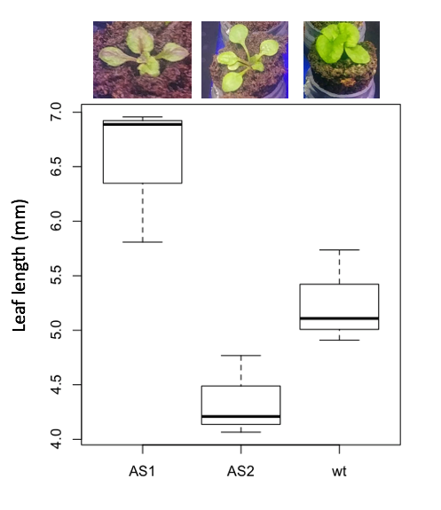
Figure 4. Box plot of lengths of leaves of a 10-day old plant from on of three strains of Arabidopsis thaliana.
4. Return to your answer to question 7 from Chapter 12.1 and review your answer and modify as appropriate to correct your language to that presented here about factors and levels.
5. Conduct the one-way ANOVA test on the Comet assay data presented question 7 from Chapter 12.1. Data are copied for your convenience to end of this page. Obtain the ANOVA table and report the value of the test statistics, degrees of freedom, and p-value.
a. Based on the ANOVA results, do you accept or reject the null hypothesis? Explain your choice.
Data used in this page
Difference, no difference
Table 12.2 Difference or No Difference
| Group | No.difference | Difference |
|---|---|---|
| A | 12.04822 | 11.336161 |
| A | 12.67584 | 13.476142 |
| A | 12.99568 | 12.96121 |
| A | 12.01745 | 11.746712 |
| A | 12.34854 | 11.275492 |
| B | 12.17643 | 7.167262 |
| B | 12.77201 | 5.136788 |
| B | 12.07137 | 6.820242 |
| B | 12.94258 | 5.318743 |
| B | 12.0767 | 7.153992 |
| C | 12.58212 | 3.344218 |
| C | 12.69263 | 3.792337 |
| C | 12.60226 | 2.444438 |
| C | 12.02534 | 2.576014 |
| C | 12.6042 | 4.575672 |
Comet assay, antioxidant properties of tea
Data presented in Chapter 12.1
Chapter 12 contents
9.3 – Yates continuity correction
Introduction
Yates continuity correction: Most statistical textbooks at this point will note that critical values in their table (or any chi-square table for that matter) are approximate, but don’t say why. We’ll make the same directive — you may need to make a correction to the for low sample numbers. It’s not a secret, so here’s why.
We need to address a quirk of the test: the chi-square distribution is a continuous function (if you plotted it, all possible values between, say, 4 and 3 are possible). But the calculated statistics we get are discrete. In our HIV-HG co-infection problem from the previous subchapter, we got what appears to be an exact answer for P, but it is actually an approximation.
We’re really not evaluating our test statistic at the alpha levels we set out. This limitation of the goodness of fit statistic can be of some consequence — increases our chance to commit a Type I error — unless we make a slight correction for this discontinuity. The good news is that the does just fine for most df, but we do get concerned with it’s performance at df = 1 and for small samples.
Therefore, the advise is to use a correction if your calculated is close to the critical value for rejection/acceptance of the null hypothesis and you have only one df. Use the Yate’s continuity correction to standard calculation,  .
.

For the 2×2 table (Table 1), we can rewrite Yates correction

Our concern is this: without the correction, Pearson’s test statistic will be biased (e.g., the test statistic will be larger than it “really” is), so we’ll end up rejecting the null hypothesis when we shouldn’t (that’s a Type I error). This becomes an issue for us when p-value is close to 5%, the nominal rejection level: what if p-value is 0.051? Or 0.049? How confident are we in concluding accept or reject null hypothesis, respectively?
I gave you three examples of goodness of fit and one contingency table example. You should be able to tell me which of these analyses it would be appropriate to apply to correction.
More about continuity corrections
Yates suggested his correction to Pearson’s back in 1934. Unsurprisingly, new approaches have been suggested (e.g., discussion in Agresti 2001). For example, Nicola Serra (Serra 2018; Serra et al 2019) introduced

Serra reported favorable performance when sample size was small and the expected value in any cell was 5 or less.
R code
When you submit a 2X2 table with one or more cells less than five, you could elect to use a Fisher exact test, briefly introduced here (see section 9.5 for additional development), or, you may apply the Yates correction. Here’s some code to make this work in R.
Let’s say the problem looks like Table 1.
Table 1. Example 2X2 table with one cell with low frequency.
| Yes | No | |
| A | 8 | 12 |
| B | 3 | 22 |
At the R prompt type the following
library(abind, pos=15)
#abind allows you to combine matrices into single arrays
.Table <- matrix(c(8,12,3,22), 2, 2, byrow=TRUE)
rownames(.Table) <- c('A', 'B')
colnames(.Table) <- c('Yes', 'No') # when you submit, R replies with the following table
.Table  # Counts
 Yes No
A  8 12
B  3 22
Here’s the command; the default is no Yates correction (i.e., correct=FALSE); to apply the Yates correction, set correct=TRUE
.Test <- chisq.test(.Table, correct=TRUE)
Output from R follows
.Test
    Pearson's Chi-squared test with Yates' continuity correction
data:  .Table
X-squared = 3.3224, df = 1, p-value = 0.06834
Compare without the Yates correction
.Test <- chisq.test(.Table, correct=FALSE)
.Test
    Pearson's Chi-squared test
data:  .Table
X-squared = 4.7166, df = 1, p-value = 0.02987
Note that we would reach different conclusions! If we ignored the potential bias of the un-corrected we would be tempted to reject the null hypothesis, when in fact, the better answer is not to reject because Yates-corrected p-value is greater than 5%.
Just to complete the work, what does the Fisher Exact test results look like (see section 9.5)?
fisher.test(.Table)
    Fisher's Exact Test for Count Data
data:  .Table
p-value = 0.04086
alternative hypothesis: true odds ratio is not equal to 1
95 percent confidence interval:
0.9130455 32.8057866
sample estimates:
odds ratio
  4.708908
Which to use? The Fisher exact test is just that, an exact test of the hypothesis. All possible outcomes are evaluated and we interpret the results as likely as p=0.04086 if there is actually no association between the treatment (A vs B) and the outcome (Yes/No) (see section 9.5).
Questions
- With respect to interpreting results from a test for small samples, why use the Yates continuity correction?
- Try your hand at the following four contingency tables (a – d). Calculate the test, with and without the Yates correction. Make note of the p-value from each and note any trends.
(a)
| Yes | No | |
| A | 18 | 6 |
| B | 3 | 8 |
(b)
| Yes | No | |
| A | 10 | 12 |
| B | 3 | 14 |
(c)
| Yes | No | |
| A | 5 | 12 |
| B | 12 | 18 |
(d)
| Yes | No | |
| A | 8 | 12 |
| B | 3 | 3 |
3. Ch09.1, Question 1 provided an example of a count from a small bag of M&Ms. Apply the Yates correction to obtain a better estimate of p-value for the problem. The data were four blue, two brown, one green, three orange, four red, and two yellow candies.
- Construct a table and compare p-values obtained with and without the Yates correction. Note any trend in p-value
Chapter 9 contents
8.5 – One sample t-test
Introduction
We’re now talking about the traditional, classical two group comparison involving continuous data types. Thus begins your introduction to parametric statistics. One sample tests involve questions like, how many — what proportion of — people would we expect are shorter or taller than two standard deviations from the mean? This type of question assumes a population and we use properties of the normal distribution and, hence, these are called parametric tests because the assumption is that the data has been sampled from a particular probability distribution.
However, when we start asking questions about a sample statistic (e.g., the sample mean), we cannot use the normal distribution directly, i.e., we cannot use Z and the normal table as we did before (Chapter 6.7). This is because we do not know the population standard deviation and therefore must use an estimate of the variation (s) to calculate the standard error of the mean.
With the introduction of the t-statistic, we’re now into full inferential statistics-mode. What we do have are estimates of these parameters. The t-test — aka Student’s t-test — was developed for the purpose of testing sample means when the true population parameters are not known.
Note 1: It’s called Student’s t-test after the pseudonym used by William Gosset.
The equation of the one sample t-test. Note the resemblance in form with the Z-score!

where  is the sample standard error of the sample mean (SEM).
For example, weight change of mice given a hormone (leptin) or placebo. The  , but under the null hypothesis, the mean change is “really” zero (
 ). How unlikely is our value of 5 g?
Note 2: Did you catch how I snuck in “placebo” and mice? Do you think the concept of placebo is appropriate for research with mice, or should we simply refer to it as a control treatment? See Ch5.4 – Clinical trials for review.
Speaking of null hypotheses, can you say (or write) the null and alternative hypotheses in this example? How about in symbolic form?
We want to know if our sample mean could have been obtained by chance alone from a population where the true change in weight was zero.
and
and we take these values and plug them into our equation of the t-test
Then recall that Degrees of Freedom are DF = n – 1 so we have DF = 20 – 1 = 19 for the one sample t-test. And the Critical Value is found in the appropriate table of critical values for the t distribution (Fig. 1)
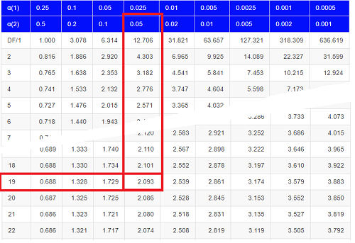
Figure 1. Table of a portion of the Critical values of the t distribution. Red selections highlight critical value for t-test at α = 5% and df = 19.
Note 3: See our table of critical values of t distribution.
Or, and better, use R
qt(c(0.025), df=19, lower.tail=FALSE)
where qt() is function call to find t-score of the pth percentile (cf 3.3 – Measures of dispersion) of the Student t distribution. For a two tailed text, we recall that 0.025 is lower tail and 0.025 is upper tail.
In this example we would be willing to reject the Null Hypothesis if there was a positive OR a negative change in weight.
This was an example of a “two-tailed test” which is “2-tail” or α(2) in Table of critical values of the t distribution.
Critical Value for α(2) = 0.05, df = 19, = 2.093
Do we accept or reject the Null Hypothesis?
A typical inference workflow
Note the general form of how the statistical test is processed, a form which actually applies to any statistical inference test.
- Identify the type of data
- State the null hypothesis (2 tailed? 1 tailed?)
- Select the test statistic (t-test) and determine its properties
- Calculate the test statistic (the value of the result of the t-test)
- Find degrees of freedom
- For the DF, get the critical value
- Compare critical value to test statistic
- Do we accept or reject the null hypothesis?
And then we ask, given the results of the test of inference, What is the biological interpretation? Statistical significance is not necessarily evidence of biological importance. In addition to statistical significance, the magnitude of the difference — the effect size — is important as part of interpreting results from an experiment. Statistical significance is at least in part because of sample size — the large the sample size, the smaller the standard error of the mean, therefore even small differences may be statistically significant, yet biologically unimportant. Effect size is discussed in Ch9.1 – Chi-square test: Goodness of fit, Ch11.4 – Two sample effect size and Ch12.5 – Effect size for ANOVA.
R Code
Let’s try a one-sample t-test. Consider the following data set: body mass of four geckos and four Anoles lizards (Dohm unpublished data).
For starters, let’s say that you have reason to believe that the true mean for all small lizards is 5 grams (g).
Geckos: 3.186, 2.427, 4.031, 1.995
Anoles: 5.515, 5.659, 6.739, 3.184
Get the data into R (Rcmdr)
By now you should be able to load this data in one of several ways. If you haven’t already entered the data, check out Part 07. Working with your own data in Mike’s Workbook for Biostatistics.
Once we have our data.frame, proceed to carry out the statistical test.
To get the one-sample t-test in Rcmdr, click on Statistics → Means → Single-sample t-test… Because there is only one numerical variable, Body.mass, that is the only one that shows up in the Variable (pick one) window (Fig 2)
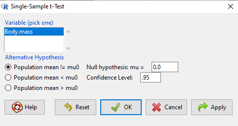
Figure 2. Screenshot Rcmdr single-sample t-test menu.
Type in the value 5.0 in the Null hypothesis =mu box.
Question 3: Quick! Can you write, in plain old English, the statistical null hypothesis???
Click OK
The results go to the Output Window.
t.test(lizards$Body.mass, alternative='two.sided', mu=5.0, conf.level=.95)
One Sample t-test
data: lizards$Body.mass
t = -1.5079, df = 7, p-value = 0.1753
alternative hypothesis: true mean is not equal to 5
95 percent confidence interval:
2.668108 5.515892
sample estimates:
mean of x 4.092
end of R output
Let’s identify the parts of the R output from the one sample t-test. R reports the name of the test and identifies
- The
dataset$variableused (lizards$Body.mass). The data set was called “lizards” and the variable was “Body.mass”. R uses the dollar sign ($) to denote the dataset and variable within the data set. - The value of the t test statistic was (t = -1.5079). It is negative because the sample mean was less than the population mean — you should be able to verify this!
- The degrees of freedom, df = 7
- The p-value = 0.1753
- 95% confidence interval of the population mean; lower limit = 2.668108, upper limit = 5.515892
- The sample mean = 4.092
Take a step back and review
Lets make sure we “get” the logic of the hypothesis testing we have just completed.
Consider the one-sample t-test.
Step 1. Define HO and HA. The null hypothesis might be that a sample mean, , is equal to μ = 5.
The alternate is that the sample mean is not equal to 20.
Where did the value 5 come from? It could be a value from the literature (does the new sample differ from values obtained in another lab?). The point is that the value is known in advance, before the experiment is conducted, and that makes it a one-sample t-test.
One tailed hypothesis or two?
We introduced you to the idea of “tails of a test” (Ch08.4). As you should recall, a null/alternate hypothesis for a two-tailed test may be written as
Null hypothesis

versus the alternative hypothesis

where is the sample mean and  is the population mean.
Alternatively, we can write one-tailed tests of null/alternate hypothesis

for the null hypothesis versus the alternate hypothesis

Question 4: Are all possible outcomes of the one-tailed test covered by these two hypotheses?
Question 5: What is the SEM for this problem?
Question 6: What is the difference between a one sample t-test and a one-sided test?
Question 7: What are some other possible hypotheses that can be tested from this simple example of two lizard species?
Step 2. Decide how certain you wish to be (with what probability) that the sample mean is different from μ. As stated previously, in biology, we say that we are willing to be incorrect 5% of the time (Cowles and Davis 1982; Cohen 1994). This means we are likely to correctly reject the null hypothesis 100% – 5% = 95% of the time, which is the definition of statistical power. We do this by setting the Type I error to be 5% (alpha, α = 0.05). The Type I error is the chance that we will reject a null hypothesis, but the true condition in the population we sampled was actually “no difference.”
Step 3. Carry out the calculation of the test statistic. In other words, get the value of t from the equation above by hand, or, if using R (yes!) simply identify the test statistic value from the R output after conducting the one sample t test.
Step 4. Evaluate the result of the test. If the value of the test statistic is greater than the critical value for the test, then you conclude that the chance (the P-value) that the result could be from that population is not likely and you therefore reject the null hypothesis.
Question 8: What is the critical value for a one-sample t-test with df = 7?
Hint; you need the table or better, use R
Rcmdr: Distributions → Continuous distributions → t distributions → t quantiles
You also need to know three additional things to answer this question.
- You need to know alpha (α), which we have said generally is set at 5%.
- You also need to know the degrees of freedom (DF) for the test. For a one sample t-test, DF = n – 1, where n is the sample size.
- You also must know whether your test is one or two-tailed.
- You then use the t-distribution (the tables of the t-distribution at the back of your book) to obtain the critical value. Note that if you use R, the actual p-value is returned.
Why learn the equations when I can just do this in R?
Rcmdr does this for you as soon as you click OK. Rcmdr returns the value of the test statistic and the p-value. R does not show you the critical value, but instead returns the probability that your test statistic is as large as it is AND the null hypothesis is true. From our one-sample t-test example, the Rcmdr output. The simple answer is that in order to understand the R output properly you need to know where each item of the output for a particual test comes from and how to interpret it. Thus, the best way is to have the equations available and to understand the algorithmic approach to statistical inference.
And, this is as good of time as any to show you how to skip the RCmdr GUI and go straight to R.
First, create your variables. At the R prompt enter the first variable
liz <- c("G","G","G","G","A","A","A","A")
and then create the second variable
bm <- c(3.186,2.427,4.031,1.995,5.515,5.659,6.739,3.184)
Next, create a data frame. Think of a data frame as another word for worksheet.
lizz <- data.frame(liz,bm)
Verify that entries are correct. At the R prompt type “lizz” wthout the quotes and you should see
lizz
 liz bm
1 G 3.186
2 G 2.427
3 G 4.031
4 G 1.995
5 A 5.515
6 A 5.659
7 A 6.739
8 A 3.184
End of R output
Carry out the t-test by typing at the R prompt the following
t.test(lizz$bm, alternative='two.sided', mu=5, conf.level=.95)
And, like the Rcmdr output we have for the one-sample t-test the following R output
One Sample t-test
data: lizards$Body.mass
t = -1.5079, df = 7, p-value = 0.1753 alternative hypothesis: true mean is not equal to 5
95 percent confidence interval:
2.668108 5.515892
sample estimates:
mean of x
4.092
End of R output
which, as you probably guessed, is the same as what we got from RCmdr.
Question 9: From the R output of the one sample t-test, what was the value of the test statistic?
- -1.5079
- 7
- 0.1753
- 2.668108
- 5.515892
- 4.092
Note. On an exam you will be given portions of statistical tables and output from R. Thus you should be able to evaluate statistical inference questions by completing the missing information. For example, if I give you a test statistic value, whether the test is one- or two-tailed, degrees of freedom, and the Type I error rate alpha, you should know that you would need to find the critical value from the appropriate statistical table. On the other hand, if I give you R output, you should know that the p-value and whether it is less than the Type I error rate of alpha would be all that you need to answer the question.
Think of this as a basic skill.
In statistics and for some statistical tests, Rcmdr and other software may not provide the information needed to decide that your test statistic is large, and a table in a statistics book is the best way to evaluate the test.
For now, double check Rcmdr by looking up the critical value from the t-table.
Check critical value against our test statistic
Df = 8 – 1 = 7
The test is two-tailed, therefore α(2)
α = 0.05 (note that two-tailed critical value is 2.365. T was equal to 1.51 (since t-distribution is symmetrical, we can ignore the negative sign), which is smaller than 2.365 and so we would agree with Rcmdr — we cannot reject the null hypothesis.
Question 10: From the R output of the one sample t-test, what was the P-value?
- -1.5079
- 7
- 0.1753
- 2.668108
- 5.515892
Question 10: We would reject the null hypothesis
- False
- True
Questions
Eleven questions were provided for you within the text in this chapter. Here’s one more.
12. Here’s a small data set for you to try your hand at the one-sample t-test and Rcmdr. The dataset contains cell counts, five counts of the numbers of beads in a liquid with an automated cell counter (Scepter, Millipore USA). The true value is 200,000 beads per milliliter fluid; the manufacturer claims that the Scepter is accurate within 15%. Does the data conform to the expectations of the manufacturer? Write a hypothesis then test your hypothesis with the one-sample t-test. Here’s the data.
| scepter |
| 258900 |
| 230300 |
| 107700 |
| 152000 |
| 136400 |
Chapter 8 contents
8.4 – Tails of a test
Introduction
The basics of statistical inference is to establish the null and alternative hypotheses. Starting with the simplest cases, where there is one sample of observations and the comparison is against a population (theory) mean, how many possible comparisons can be made? The next simplest is the two-sample case, where we have two sets of observations and the comparison is against the two groups. Again, how many total comparisons may be made?
Let , “X bar”, equal the sample mean and , “mu”, represent the population mean. For sample means, designate groups by a subscript, 1 or 2. We then have Table 1.
Table 1. Possible hypothesis involving two groups
| Comparison | One-same | Two-sample |
| 1. |  |
 |
| 2. |  |
 |
| 3. |  |
 |
| 4. |  |
 |
| 5. |  |
 |
| 6. |  |
 |
Classical statistics classifies inference into null hypothesis, HO, vs. alternate hypotheses, HA, and specifies that we test null hypotheses based on the value of the estimated test statistic (see discussion about critical value and p-value, Chapter 8.2). From the list of six possible comparisons we can divide them into one-tailed and two-tailed differences (Table 1). By “tail” we are referring to the ends or tails of a distribution (Figure 1, Figure 2); where do our results fall on the distribution?
Two-tailed hypotheses: Comparison 1 and comparison 2 in the table above are two-tailed hypotheses. We don’t ask about the direction of any difference (less than or greater than).
Figure 1 shows the “two-tailed” distribution — if our results fall to the left ,  , or to the right
  we reject the null hypothesis (blue regions in the curve). We divide the type I error into two equal halves.
Note. It’s a nice trick to shade in regions of the curve. A package tigerstats includes the function pnormGC that simplifies this task.
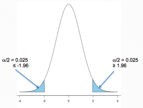
Figure 1. Two-tailed distribution.
library(tigerstats)
pnormGC(c(-1.96,1.96), region="outside", mean=0, sd=1,graph=TRUE)
Figure 2 shows the “one-tailed” distribution — if our alternate hypothesis was that the sample mean was less than the population mean, then our fall to the left,  , for the “lower tail” of the distribution. If, however, our alternate hypothesis was that the sample mean was greater than the population mean, then our region of interest falls to the right,
  . Again, we reject the null hypothesis (blue regions in the curve). Note for one-tailed hypothesis, all Type I error occurs in the one area, not both, so
  (alpha) remains 0.05 over the entire rejection region (Fig 2).
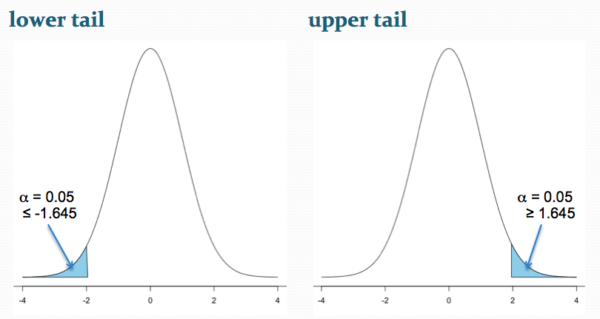
Figure 2. One-tailed distribution, lower tail (left) and upper tail (right).
library(tigerstats)
pnormGC(1.645, region="above", mean=0, sd=1,graph=TRUE)
pnormGC(-1.645, region="below", mean=0, sd=1,graph=TRUE)
One-tailed hypotheses: Comparison 3 through comparison 6 in the table are one-tailed hypotheses. The direction of the difference matters.
Note a simple trick to writing one-tailed hypotheses: first write the alternate hypothesis because the null hypothesis includes all of the other possible outcomes of the test.
Examples
Lets consider some examples. We learn best by working through cases.
Chemotherapy as an approach to treat cancers owes its origins to the work of Dr Sidney Farber among others in the 1930s and ’40s (DeVita and Chu 2008; Mukherjee 2011). Following up on the observations of others that folic acid (vitamin B9) improved anemia, Dr Farber believed that folic acid might reverse the course of leukemia (Mukherjee 2011). In 1946 he recruited several children with acute lymphoblastic leukemia and injected them with folic acid. Instead of ameliorating their symptoms (e.g., white blood cell counts and percentage of abnormal immature white blood cells, called blast cells), treatments accelerated progression of the disease. That’s a scientific euphemism for the reality — the children died sooner in Dr. Faber’s trial than patients not enrolled in his study. He stopped the trials. Clearly, adding folic acid was not a treatment against this leukemia.
Question 1. Do you think these experiments are one sample or two sample? Hint: Is there mention of a control group?
Answer: There’s no mention of a control group, but instead, Dr. Faber would have had plenty of information about the progression of this disease in children. This was a one sample test.
Question 2. What would be a reasonable interpretation of Dr Faber’s alternate hypothesis with respect to percentage of blast cells in patients given folic acid treatment? Your options are
- Folic acid supplementation has an effect on blast counts.
- Folic acid supplementation reduces blast counts.
- Folic acid supplementation increases blast counts.
- Folic acid supplementation has no effect on blast counts.
Answer: At the start of the trials, it is pretty clear that the alternate hypothesis was intended to be a one-tailed test (option 2). Dr. Faber’s alternative hypothesis clearly was that he believed that addition of folic acid would reduce blast cell counts. However, that they stopped the trials shows that they recognized that the converse had occurred, that blast counts increased; this means that, from a statistician’s point of view, Dr Faber’s team was testing a two-sided hypothesis (option 1).
Another example.
Dr Farber reasoned that if folic acid accelerated leukemia progression, perhaps anti-folic compounds might inhibit leukemia progression. Dr Farber’s team recruited patients with acute lymphoblastic leukemia and injected them with a folic acid agonist called aminopterin. Again, he predicted that blast counts would reduce following administration of the chemical. This time, and for the first time in recorded medicine, blast counts of many patients drastically reduced to normal levels and the patients experienced remissions. The remissions were not long lasting and all patients eventually succumbed to leukemia. Nevertheless, these were landmark findings — for the first time a chemical treatment was shown to significantly reduce blast cell counts, even leading to remission, if however brief (Mukherjee 2011).
Try Question 3 and Question 4 yourself.
Question 3. Do you think these experiments are one sample or two sample? Hint: Is there mention of a control group?
Question 4. What would be a reasonable interpretation of Dr Faber’s alternate hypothesis with respect to percentage of blast cells in patients given aminopterin treatment? Your options are
- Aminopterin supplementation has an effect on blast counts.
- Aminopterin supplementation reduces blast counts.
- Aminopterin supplementation increases blast counts.
- Aminopterin supplementation has no effect on blast counts.
Pros and Cons to One-sided testing
Here’s something to consider: why not restrict yourself to one-tailed hypotheses? Here’s the pro-argument. Strictly speaking you gain statistical power to test the null hypothesis. For example, look up the t-test distribution for degrees of freedom equal to 20 and compare  (one tail) vs.
  (two-tail). You will find that for the one-tailed test, the critical value of the t-distribution with 20 df is 1.725, whereas for the two-tailed test, the critical value of the t-distribution with the same numbers of df is 2.086. Thus, the difference between means can be much smaller in the one-tailed test and prove to be “statistically significant.” Put simply, with the same data, we will reject the Null Hypothesis more often with one-tailed tests.
The con-argument. If you use a one-tailed test you MUST CLEARLY justify its use and be aware that a deviation in the opposite direction MUST be ignored! More specifically, you interpret a one-tailed result in the opposite direction as acceptance of the null — you cannot, after the fact, change your mind and start speaking about “statistically significant differences” if you had specified a one-tailed hypothesis and the results showed differences in the opposite direction.
Note. Recall also that, by itself, statistical significance judged by the p-value against a specified cut-off critical value is not enough to say there is evidence for or against the hypothesis. For that we need to consider effect size, see Power analysis in Chapter 11.
Questions
- For a Type I error rate of 5% and the following degrees of freedom, compare the critical values for one tail test and a two tailed test of the null hypothesis.
- 5 df
- 10 df
- 15 df
- 20 df
- 25 df
- 30 df
- Using your findings from Additional Question 1, make a scatterplot with degrees of freedom on the horizontal axis and critical values on the vertical axis. What trend do you see for the difference between one and two tailed tests as degrees of freedom increase?
- A clinical nutrition researcher wishes to test the hypothesis that a vegan diet lowers total serum cholesterol levels compared to an omnivorous diet. What kind of hypothesis should he use, one-tailed or two-tailed? Justify your choice.
- Spironolactone, introduced in 1953, is used to block aldosterone in hypertensive patients. A newer drug eplerenone, approved by the FDA in 2002, is reported to have the same benefits as spironolactone (reduced mortality, fewer hospitalization events), but with fewer side effects compared with spironolactone. Does this sentence suggest a one-tailed test or a two-tailed test?
- Write out the appropriate null and alternative hypothesis statements for the spironolactone and eplerenone scenario.
- You open up a bag of Original Skittles and count the number of green, orange, purple, red, and yellow candies in the bag. What kind of hypothesis should be used, one-tailed or two-tailed? Justify your choice.
- Verify the probability values from the table of standard normal distribution for Z equal to -1.96, -1.645, 1.645, and 1.96.
Chapter 8 contents
8.2 – The controversy over proper hypothesis testing
Introduction
Over the next several chapters we will introduce and develop an approach to statistical inference, which has been given the title “Null Hypothesis Significance Testing” or NHST.
In outline, NHST proceeds with
- statements of two hypotheses, a null hypothesis, HO, and an alternative hypothesis, HA
- calculate a test statistic comparison of the null hypothesis (assuming some characteristic of data).
- The value of the test statistic is to be compared to a critical value for the test, identified for the assumed probability distribution at associated degrees of freedom for the statistical function, and assigned Type I error rate.
We will expand on these statements later in this chapter, so stay with me here. Basically, the null hypothesis is often a statement like the responses of subjects from the treatment and control groups are the same, e.g., no treatment effect. Note that the alternative hypothesis, e.g., hypertensive patients receiving hydalazine for six weeks have lower systolic blood pressure than patients receiving a placebo (Campbell et al 2011), would be the scientific hypothesis we are most interested in. But in the Frequentist NHST approach we test the null hypothesis, not the alternative hypothesis. This framework over proper hypothesis testing is the basis of the Bayesian vs Frequentist controversy.
Consider the independent sample t-test (see Chapter 8.5 and 8.6), our first example of a parametric test.

After plugging in the sample means and the standard error for the difference between the means, we calculate t, the test statistic of the t-test. The critical value is treated as a cut-off value in the NHST approach. We have to set our Type I error rate before we start the experiment, and we have available the degrees of freedom for the test, which follows from the sample size. With these in hand, the critical value is found by looking in the t-table of probabilities (or better, use R).
For example, what is the critical value of t-test with 10 degrees of freedom and Type I error of 5%?
In Rcmdr, choose Distributions → Continuous distributions → t distribution → t quantiles…
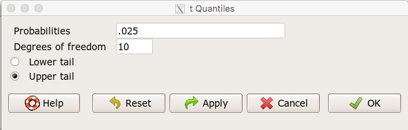
Figure 1. Screenshot t-quantiles Rcmdr
Note we want Type I equal to 5%. Since their are two tails for our test, we divide 5% by two and enter 0.025 and select the Upper tail.
R output
> qt(c(.025), df=10, lower.tail=FALSE)
[1] 2.228139
which is the same thing we would get if we look up on the t-distribution table (Fig. 2).
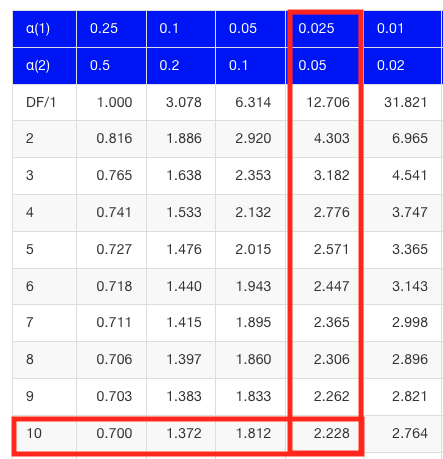
Figure 2. Screenshot of portion of t-table with highlighted (red) critical value for 10 degrees of freedom.
If the test statistic is greater than the critical value, then the conclusion is that the null hypothesis is to be provisionally rejected. We would like to conclude that the alternative hypothesis should favored as best description of the results. However, we cannot — the p-value simply tells us how likely our results would be obtained and if the null hypothesis was true. Confusingly, however, you cannot interpret the p-value as telling you the probability (how likely) that the null hypothesis is true. If however the test statistic is less than the critical value, then the conclusion is that the null hypothesis is to be provisionally accepted.
The test statistic can be assigned a probability or p-value. This p-value is judged to be large or small relative to an a priori error probability level cut off called the Type I error rate. Thus, NHST as presented in this way may be thought of as a decision path — if the test statistic is greater than the critical value, which will necessarily mean that the p value is less than the Type I error rate, then we make one type of conclusion (reject HO). In contrast, if the test statistic is less than the critical value, which will mean that the p-value associated with the test statistic will be greater than the Type I error rate, then we conclude something else about the null hypothesis. The various terms used in this description of NHST were defined in Chapter 8.3.
Sounds confusing, but, you say, OK, what exactly is the controversy? The controversy has to do whether the probability or p-value can be interpreted as evidence for a hypothesis. In one sense, the smaller the p-value, the stronger the case to reject the null hypothesis, right? However, just because the p-value is small — the event is rare — how much evidence do we have that the null hypothesis is true? Not necessarily, and so we can only conclude that the p-value is one part of what we may need for evidence for or against a hypothesis (hint: part of the solution is to consider effect size — introduced in Chapter 9.2 — and the statistical power of the test, see Ch 11). What follows was covered by Goodman (1988) and others. Here’s the problem. Consider tossing a fair coin ten times, with the resulting trial yielding nine out of ten heads (e.g., a value of one, with tails equal to zero).
R code
set.seed(938291156)
rbinom(10,1,0.5)
[1] 1 1 1 1 1 1 0 1 1 1
Note 1: To get this result I repeated rbinom() a few times until I saw this rare result. I then used the command get_seed() from mlr3misc package to retrieve current seed of R’s random number generator. Initialize the random seed with the command set.seed().
While rare (binomial probability 0.0098), do we take this as evidence that the coin is not fair? By itself, the p-value provides no information about the alternative hypothesis. More about p-value follows below in sections What’s wrong with the p-value from NHST? and The real meaning and interpretation of P-values.
Statisticians have been aware of limitations of the NHST approach for years (see editorial by Wasserstein et al 2019), but only now is the message getting attention of researchers in the biosciences and other fields. In fact, the New York Times recently had a nice piece by F.D. Flam (“The Odds, Continually Updated,” 29 Sep 2014) on the controversy and the Bayesian alternative. Like most controversies there are strong voices on either side, and it can be difficult as an outsider to know which position to side with (Fig. 3).
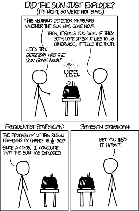
Figure 3. xkcd: Frequentists vs. Bayesians, https://xkcd.com/1132/
The short answer is — as you go forward do realize that there is a limitation to the frequentist approach and to be on the correct side of the controversy, you need to understand what you can conclude from statistical results. NHST is by far the most commonly used approached in biosciences (e.g., out of 49 research articles I checked from four randomly selected issues of 2015 PLoS Biology, 43 used NHST, 2 used a likelihood approach, none used Bayesian statistics). The NHST is also the overwhelming manner in which we teach introductory statistics courses (e.g., checking out the various MOOC courses at www.coursera.org, all of the courses related to Basic Statistics or Inferential Statistics are taught primarily from the NHST perspective). However, right from the start I want to emphasize the limits of the NHST approach.
If the purpose of science is to increase knowledge, then the NHST approach by itself is an inadequate framework at best, and in the eyes of some, worthless! Now, I think this latter sentiment is way over the top, but there is a need for us to stop before we begin, in effect, to set the ground rules for what can be interpreted from the NHST approach. The critics of NHST have a very important point, and that needs to be emphasized, but we will also defend use and teaching of this approach so that you are not left with the feeling that somehow this is a waste of time or that you are being cheated from learning the latest knowledge on the subject of statistical inference. The controversy hinges on what probability means.
P-values, statistical power, and replicability of research findings
Science, as a way of knowing how the world works, is the only approach that humans have developed that has been empirically demonstrated to work. Note how I narrowed what science is good for — if we are asking questions about the material world, then science should be your toolkit. Some (e.g., Platt 1964), may further argue that there are disciplines in science that have been more successful (e.g., molecular biology) than others (e.g., evolutionary psychology, cf discussion in Ryle 2006) at advancing our knowledge about the material world. However, to the extent research findings are based solely on statistical results there is reason to believe that many studies in fact have not recovered truth (Ioannidis 2005). In a review of genomics, it was reported that findings of gene expression differences by many microarray studies were not reproducible (Allison et al 2006). The consensus is that confidence in the findings should hold only for the most abundant gene transcripts of many microarray gene expression profiling studies, a conclusion that undercuts the perceived power of the technology to discover new causes of disease and the basis for individual differences for complex phenotypes. Note that when we write about failure of research reproducibility we are not including cases of alleged fraud (Carlson 2012 on Duke University oncogenomics case), we are instead highlighting that these kinds of studies often lack statistical power; hence, when repeated, the experiments yield different results.
Frequentist and Bayesian Probabilities
Turns out there is a lot of philosophical problems around the idea of “probability,” and three schools of thought. In the Fisherian approach to testing, the researcher devises a null hypothesis, HO, collects the data, then computes a probability (p-value) of the result or outcome of the experiment. If the p-value is small, then this is inferred as little evidence in support of the null hypothesis. In the Frequentists’ approach, the one we are calling NHST, the researcher devises two hypotheses, the null hypothesis, HO, and an alternative hypothesis, HA. The results are collected from the experiment and, prior to testing, a Type I error rate (α, chance) is defined. The Type I error rate is set to some probability and refers to the chance of rejecting the null hypothesis purely due to random chance. The Frequentist then computes a p-value of result of the experiment and applies a decision criterion: If P-value greater than Type I error rate, then provisionally accept null hypothesis. In both the Fisherian and Frequentist approaches, the probability, again defined at the relative frequency of an event over time, is viewed as a physical, objective and well-defined set of values.
Bayesian approach: based on Bayes conditional probability, one identifies the prior (subjective) probability of an hypothesis, then, adjusts the prior probability (down or up) as new results come in. The adjusted probability is known as posterior probability and it is equal to the likelihood function for the problem. The posterior probability is related to the prior probability and this function can be summarized by the Bayes factor as evidence the evidence against the null hypothesis. And that’s what we want, a metric of our evidence for or against the null hypothesis.
Note 2: A probability distribution function (PDF) is a function of the sample data and returns how likely that particular point will occur in the sample. The distribution is given. The likelihood function approaches this from a different direction. The likelihood function takes the data set as a given and represents how likely are the different parameters for your distribution.
We can calibrate the Bayesian probability to the frequentist p-value (Selke et al 2001; Goodman 2008; Held 2010; Greenland and Poole 2012). Methods to achieve this calibration vary, but the Fagan nomogram Held (2010) proposed is a good tool for us as we go forward. We can calculate our NHST p-value, but then convert the p-value to a Bayes factor by looking at the nomogram. I mention this here not as part of your to do list, but rather as a way past the controversy: the NHST p-value can be transcribed to a Bayesian conditional probability.
Likelihood
Before we move on there is one more concept to introduce, that of likelihood. We describe a model (an equation) we believe can generate the data we observe. By constructing different models with different parameters (hypotheses), you generate a statistic that yields a likelihood value. If the model fits the data, then the likelihood function has a small value. The basic idea then is to compare related, but different models to see which fits the data better. We will use this approach when comparing linear models when we introduce multiple regression models in Chapter 18.
What’s wrong with the p-value from NHST?
Well, really nothing is “wrong” with the p-value.
Where we tend to get into trouble with the p-value concept is when we try and interpret it. See below, Why is this important to me as a beginning student? The p-value is not evidence for a position, it is a statement about error rates. The p-value from NHST can be viewed as the culmination of a process that is intended to minimize the chance that the statistician makes an error.
In Bayesian terms, the p-value from NHST is the probability that we observe the data (e.g., the differences between two sample means), assuming the null hypothesis is true. If we want to interpret the p-value in terms of evidence for a proposition, then we want the conditional error probability.
Sellke et al (2001) provided a calibration of p-values and, assuming that the prior probabilities of the null hypothesis and the alternative hypothesis are equal (that is, that each have a prior probability of 0.5), by using a formula provided by them (equation 3), we can correct our NHST p-value into a probability that can be interpreted as evidence in favor of the interpretation that the null hypothesis is true. In Bayesian terms this is called the posterior probability of the null hypothesis. The formula is
![\begin{align*} conditional \ error \ probability =\left \{ 1+ \left ( -e \cdot p \cdot ln \left [ p \right ]^{-1}\right )\right \}^{-1} \end{align*}](https://biostatistics.letgen.org/wp-content/ql-cache/quicklatex.com-09e06b0ea028cc8cfaf82e8001b59ad1_l3.png "Rendered by QuickLaTeX.com")
where e is Euler’s number, the base of the natural logarithm (ln), and p is the p-value from the NHST. This calibration works as long as  (Sellke et al 2001).
By convention we set the Type I error at 5% (cf Cohen 1994). How strong of evidence is a p-value near 5% against the null hypothesis being true, again, under the assumption that the prior probability of the null hypothesis being true is 50%? Using the above formula I constructed a plot of the calculated conditional error probability values against p-values (Fig. 4).
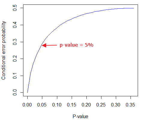
Figure 4. Conditional error probability values plotted against p-values.
As you can see, a p-value of 5% is not strong evidence at just 0.289. Not until p-values are smaller than 0.004 does the conditional error probability value dip below 0.05, suggesting strong evidence against the null hypothesis being true.
R note: For those of you keeping up with the R work, here’s the code for generating this plot. Text after “#” are comments and are not interpreted by R.
At the R prompt type each line
NHSTp = seq(0.00001,0.37,by=0.01)      #create a sequence of numbers between 0.0001 and 0.37 with a step of 0.01
CEP = (1+(-1*exp(1)*NHSTp*log(NHSTp))^-1)^-1    #equation 3 from Sellke et al 2001
plot(NHSTp,CEP,xlab="P-value", ylab="Conditional error probability",type="l",col="blue")
Why is this important to me as a beginning student?
As we go forward I will be making statements about p-values and Type I error rates and null hypotheses and even such things as false positives and false negative. We need to start to grapple with what exactly can be said by p-values in the context of statistical inference, and to recognize that we will sometimes state conclusions that cut some corners when it comes to interpreting p-values. And yet, you (and all consumers of statistics!) are expected to recognize what p-values mean. Always.
The real meaning and interpretation of P-values
This is as good of a time as any to make some clarification about the meaning of p-value and the whole inference concept. Fisher indeed came up with the concept of the p-value, but its use as a decision criterion owes to others and Fisher disagreed strongly with use of the p-value in this way (Fisher 1955; Lehmann 1993).
Here are some common p-value corner-cutting statements to avoid using (after Goodman 2008; Held 2010). P-values are sometimes interpreted, incorrectly, as
Table. Incorrect interpretations of NHST p-values
- the probability of obtaining the observed data under the assumption of no real effect
- an observed type-I error rate
- the false discovery rate, i.e. the probability that a significant finding is a “false positive”
- the (posterior) probability of the null hypothesis.
So, if p-values don’t mean any of these things, what does a p-value mean? It means that we begin by assuming that there is no effect of our treatments — the p-value is then the chance we will get as large of a result (our test statistic) and the null hypothesis is true. Note that this definition does not include a statement about evidence of the null hypothesis being true. To get evidence of “truth” we need additional tools, like the Bayes Factor and the correction of the p-value to the conditional error probability (see above). Why not dump all of the NHST and go directly to a Bayesian perspective, as some advise? The single best explanation was embedded in the assumption we made about the prior probability in order to calculate the conditional error probability. We assumed the prior probability was 50%. For many, many experiments, that is simply a guess. The truth is we generally don’t know what the prior probability is. Thus, if this assumption is incorrect, then the justification for the formula by Sellke et al (2001) is weakened, and we are no closer to establishing evidence than before. The take home message is that it is unlikely that a single experiment will provide strong evidence for the truth. Thus the message is repeat your experiments — and you already knew that! And the Bayesians can tell us that with the addition of more and more data reduces the effect of the particular value of the prior probability on our calculation of the conditional error probability. So, that’s the key to this controversy over the p-value.
Reporting p-values
Estimated p-values can never be zero. Students may come to use software that may return p-values like “0” — I’m looking at you Google Sheets re: default results from CHISQ.TEST() — but again, this does not mean the probability of the result is zero. The software simply reports values to two significant figures and failed to round. Some journals may recommend that 0 should be replaced by p < 0.01 or even < 0.05 inequalities, but the former lacks precision and the latter over-emphasizes the 5% Type I error rate threshold, the “statistical significance” of the result. In general, report p-value to three significant figures and four digits. If a p-value is small, use scientific notation and maintain significant digits. Thus, a p-value of 0.004955794 should be reported as 0.00496 and a p-value of 0.0679 should be reported as 0.0679. Use R’s signif() function, for example p-value reported as 6.334e-05, then
signif(6.334e-05,3)
[1] 6.33e-05
Rounding and significant figures were discussed in Chapter 3.5. See Land and Altman (2015) for guidelines on reporting p-values and other statistical results.
Questions
- Revisit Figure 1 again and consider the following hypothesis — the sun will rise tomorrow.
- If we take the Frequentist position, what would the null hypothesis be?
- If we take the Bayesian approach, identify the prior probability.
- Which approach, Bayesian or Frequentist, is a better approach for testing this hypothesis?
- Consider the pediatrician who, upon receiving a chest X-ray for a child notes the left lung has a large irregular opaque area in the lower quadrant. Based on the X-ray and other patient symptoms, the doctor diagnoses pneumonia and prescribes a broad-spectrum antibiotic. Is the doctor behaving as a Frequentist or a Bayesian?
- With the p-value interpretations listed in the table above in hand, select an article from PLoS Biology, or any of your other favorite research journals, and read how the authors report results of significance testing. Compare the precise wording in the results section against the interpretative phrasing in the discussion section. Do the authors fall into any of the p-value corner-cutting traps?
Chapter 8 contents
- Introduction
- The null and alternative hypotheses
- The controversy over proper hypothesis testing<.span>
- Sampling distribution and hypothesis testing
- Tails of a test
- One sample t-test
- Confidence limits for the estimate of population mean
- References and suggested readings
8.1 – The null and alternative hypotheses
Introduction
Classical statistical parametric tests — t-test (one sample t-test, independent sample-t-test), analysis of variance (ANOVA), correlation, and linear regression— and nonparametric tests like  (chi-square: goodness of fit and contingency table), share several features that we need to understand. It’s natural to see all the details as if they are specific to each test, but there’s a theme that binds all of the classical statistical inference in order to make claim of “statistical significance.”
- a calculated test statistic
- degrees of freedom associated with the calculation of the test statistic
- a probability value or p-value which is associated with the test statistic, assuming a null hypothesis is “true” in the population from which we sample.
- Recall from our previous discussion (Chapter 8.2) that this is not strictly the interpretation of p-value, but a short-hand for how likely the data fit the null hypothesis. P-value alone can’t tell us about “truth.”
- in the event we reject the null hypothesis, we provisionally accept the alternative hypothesis.
Statistical Inference in the NHST Framework
By inference we mean to imply some formal process by which a conclusion is reached from data analysis of outcomes of an experiment. The process at its best leads to conclusions based on evidence. In statistics, evidence comes about from the careful and reasoned application of statistical procedures and the evaluation of probability (Abelson 1995).
Formally, statistics is rich in inference process (Bzdok et al, 2018). We begin by defining the classical frequentist, aka Neyman-Pearson approach, to inference, which involves the pairing of two kinds of statistical hypotheses: the null hypothesis (HO) and the alternate hypothesis (HA). The null hypothesis assumes that any observed difference between the groups are the results of random chance (introduced in Ch 2.3 – A brief history of (bio)statistics ), where “random chance” implies that outcomes occur without order or pattern (Eagle 2021). Whether we reject or accept the null hypothesis — a short-hand for the more appropriate “provisionally reject” in light of the humility that our results may reflect a rare sampling event — based on the outcome of our statistical inference, the inference is evaluated against a decision criterion (cf discussion in Christiansen 2005), a fixed statistical significance level (Lehmann 1992). Significance level refers to the setting of a p-value threshold before testing is done. The threshold is often set to Type I error of 5% (Cowles & Davis 1982), but researchers should always consider whether this threshold is appropriate for their work (Benjamin et al 2017).
This inference process is referred to as Null Hypothesis Significance Testing, NHST. Additionally, a probability value will be obtained for the test outcome or test statistic value. In the Fisherian likelihood tradition, the magnitude of this statistic value can be associated with a probability value, the p-value, of how likely the result is given the null hypothesis is “true”. (Again, keep in mind that this is not strictly the interpretation of p-value, it’s a short-hand for how likely the data fit the null hypothesis. P-value alone can’t tell us about “truth”, per our discussion, Chapter 8.2.)
Note 1: About -logP. P-values are traditionally reported as a decimal, like 0.000134, in the closed (set) interval (0,1) — p-values can never be exactly zero or one. The smaller the value, the less the chance our data agree with the null prediction. Small numbers like this can be confusing, particularly if many p-values are reported, like in many genomics works, e.g., GWAS studies. Instead of reporting vanishingly small p-values, studies may report the negative log10 p-value, or -logP. Instead of small numbers, large numbers are reported, the larger, the more against the null hypothesis. Thus, our p-value becomes 3.87 -logP.
R code
-1*log(0.000134,10)
[1] 3.872895
Why log10 and not some other base transform? Just that log10 is convenience — powers of 10.
The antilog of 3.87 returns our p-value
> 10^(-1*3.872895)
[1] 0.0001340001
For convenience, a partial p-value -logP transform table
| P-value | -logP |
| 0.1 | 1 |
| 0.01 | 2 |
| 0.001 | 3 |
| 0.0001 | 4 |
On your own, complete the table up to -logP 5 – 10. See Question 7 below.
NHST Workflow
We presented in the introduction to Chapter 8 without discussion a simple flow chart to illustrate the process of decision (Figure 1). Here, we repeat the flow chart diagram and follow with descriptions of the elements.
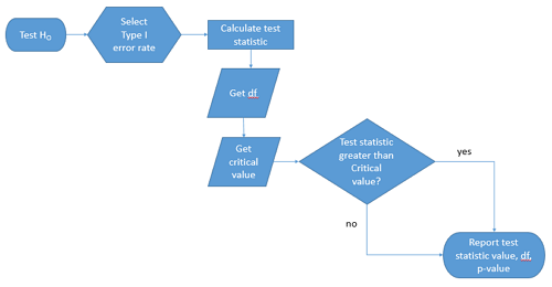
Figure 1. Flow chart of inductive statistical reasoning.
What’s missing from the flow chart is the very necessary caveat that interpretation of the null hypothesis is associated with two kinds of error, Type I error and Type II error. These points and others are discussed in the following sections.
We start with the hypothesis statements. For illustration we discuss hypotheses in terms of comparisons involving just two groups, also called two sample tests. One sample tests in contrast refer to scenarios where you compare a sample statistic to a population value. Extending these concepts to more than two samples is straight-forward, but we leave that discussion to Chapters 12 – 18.
Null hypothesis
By far the most common application of the null hypothesis testing paradigm involves the comparisons of different treatment groups on some outcome variable. These kinds of null hypotheses are the subject of Chapters 8 through 12.
The Null hypothesis (HO) is a statement about the comparisons, e.g., between a sample statistic and the population, or between two treatment groups. The former is referred to as a one tailed test whereas the latter is called a two-tailed test. The null hypothesis is typically “no statistical difference” between the comparisons.
For example, a one sample, two tailed null hypothesis.

and we read it as “there is no statistical difference between our sample mean and the population mean.” For the more likely case in which no population mean is available, we provide another example, a two sample, two tailed null hypothesis.

Here, we read the statement as “there is no difference between our two sample means.” Equivalently, we interpret the statement as both sample means estimate the same population mean.

Under the Neyman-Pearson approach to inference we have two hypotheses: the null hypothesis and the alternate hypothesis. The hull hypothesis was defined above.
Note 2: Tails of a test are discussed further in chapter 8.4.
Alternative hypothesis
Alternative hypothesis (HA): If we conclude that the null hypothesis is false, or rather and more precisely, we find that we provisionally fail to reject the null hypothesis, then we provisionally accept the alternative hypothesis. The view then is that something other than random chance has influenced the sample observations. Note that the pairing of null and alternative hypotheses covers all possible outcomes. We do not, however, say that we have evidence for the alternative hypothesis under this statistical regimen (Abelson 1995). We tested the null hypothesis, not the alternative hypothesis. Thus, it is incorrect to write that, having found a statistical difference between two drug treatments, say aspirin and acetaminophen for relief of migraine symptoms, it is not correct to conclude that we have proven the case that acetaminophen improves improves symptoms of migraine sufferers.
For the one sample, two tailed null hypothesis, the alternative hypothesis is

and we read it as “there is a statistical difference between our sample mean and the population mean.” For the two sample, two tailed null hypothesis, the alternative hypothesis would be

and we read it as “there is a statistical difference between our two sample means.”
Alternative hypothesis often may be the research hypothesis
It may be helpful to distinguish between technical hypotheses, scientific hypothesis, or the equality of different kinds of treatments. Tests of technical hypotheses include the testing of statistical assumptions like normality assumption (see Chapter 13.3) and homogeneity of variances (Chapter 13.4). The results of inferences about technical hypotheses are used by the statistician to justify selection of parametric statistical tests (Chapter 13). The testing of some scientific hypothesis like whether or not there is a positive link between lifespan and insulin-like growth factor levels in humans (Fontana et al 2008), like the link between lifespan and IGFs in other organisms (Holtzenberger et al 2003), can be further advanced by considering multiple hypotheses and a test of nested hypotheses and evaluated either in Bayesian or likelihood approaches (Chapter 16 and Chapter 17).
How to interpret the results of a statistical test
Any number of statistical tests may be used to calculate the value of the test statistic. For example, a one sample t-test may be used to evaluate the difference between the sample mean and the population mean (Chapter 8.5) or the independent sample t-test may be used to evaluate the difference between means of the control group and the treatment group (Chapter 10). The test statistic is the particular value of the outcome of our evaluation of the hypothesis and it is associated with the p-value. In other words, given the assumption of a particular probability distribution, in this case the t-distribution, we can associate a probability, the p-value, that we observed the particular value of the test statistic and the null hypothesis is true in the reference population.
By convention, we determine statistical significance (Cox 1982; Whitley & Ball 2002) by assigning ahead of time a decision probability called the Type I error rate, often given the symbol α (alpha). The practice is to look up the critical value that corresponds to the outcome of the test with degrees of freedom like your experiment and at the Type I error rate that you selected. The Degrees of Freedom (DF, df, or sometimes noted by the symbol v), are the number of independent pieces of information available to you. Knowing the degrees of freedom is a crucial piece of information for making the correct tests. Each statistical test has a specific formula for obtaining the independent information available for the statistical test. We first were introduced to DF when we calculated the sample variance with the Bessel correction, n – 1, instead of dividing through by n. With the df in hand, the value of the test statistic is compared to the critical value for our null hypothesis. If the test statistic is smaller than the critical value, we fail to reject the null hypothesis. If, however, the test statistic is greater than the critical value, then we provisionally reject the null hypothesis. This critical value comes from a probability distribution appropriate for the kind of sampling and properties of the measurement we are using. In other words, the rejection criterion for the null hypothesis is set to a critical value, which corresponds to a known probability, the Type I error rate.
Before proceeding with yet another interpretation, and hopefully less technical discussion about test statistics and critical values, we need to discuss the two types of statistical errors. The Type I error rate is the statistical error assigned to the probability that we may reject a null hypothesis as a result of our evaluation of our data when in fact in the reference population, the null hypothesis is, in fact, true. In Biology we generally use Type I error α = 0.05 level of significance. We say that the probability of obtaining the observed value AND HO is true is 1 in 20 (5%) if α = 0.05. Put another way, we are willing to reject the Null Hypothesis when there is only a 5% chance that the observations could occur and the Null hypothesis is still true. Our test statistic is associated with the p-value; the critical value is associated with the Type I error rate. If and only if the test statistic value equals the critical value will the p-value equal the Type I error rate.
The second error type associated with hypothesis testing is, β, the Type II statistical error rate. This is the case where we accept or fail to reject a null hypothesis based on our data, but in the reference population, the situation is that indeed, the null hypothesis is actually false.
Thus, we end with a concept that may take you a while to come to terms with — there are four, not two possible outcomes of an experiment.
Outcomes of an experiment
What are the possible outcomes of a comparative experiment\? We have two treatments, one in which subjects are given a treatment and the other, subjects receive a placebo. Subjects are followed and an outcome is measured. We calculate the descriptive statistics aka summary statistics, means, standard deviations, and perhaps other statistics, and then ask whether there is a difference between the statistics for the groups. So, two possible outcomes of the experiment, correct\? If the treatment has no effect, then we would expect the two groups to have roughly the same values for means, etc., in other words, any difference between the groups is due to chance fluctuations in the measurements and not because of any systematic effect due to the treatment received. Conversely, then if there is a difference due to the treatment, we expect to see a large enough difference in the statistics so that we would notice the systematic effect due to the treatment.
Actually, there are four, not two, possible outcomes of an experiment, just as there were four and not two conclusions about the results of a clinical assay. The four possible outcomes of a test of a statistical null hypothesis are illustrated in Table 1.
Table 1. When conducting hypothesis testing, four outcomes are possible.
| HO in the population | |||
| True | False | ||
| Result of statistical test | Reject HO | Type I error with probability equal to
α (alpha) |
Correct decision, with probability equal to
1 – β (1 – beta) |
| Fail to reject the HO | Correct decision with probability equal to
1 – α (1 – alpha) |
Type II error with probability equal to
β (beta) |
|
In the actual population, a thing happens or it doesn’t. The null hypothesis is either true or it is not. But we don’t have access to the reference population, we don’t have a census. In other words, there is truth, but we don’t have access to the truth. We can weight, assigned as a probability or p-value, our decisions by how likely our results are given the assumption that the truth is indeed “no difference.”
If you recall, we’ve seen a table like Table 1 before in our discussion of conditional probability and risk analysis (Chapter 7.3). We made the point that statistical inference and the interpretation of clinical tests are similar (Browner and Newman 1987). From the perspective of ordering a diagnostic test, the proper null hypothesis would be the patient does not have the disease. For your review, here’s that table (Table 2).
Table 2. Interpretations of results of a diagnostic or clinical test.
| Does the person have the disease\? | |||
| Yes | No | ||
| Result of the diagnostic test |
Positive | sensitivity of the test (a) | False positive (b) |
| Negative | False negative (c) | specificity of the test (d) | |
Thus, a positive diagnostic test result is interpreted as rejecting the null hypothesis. If the person actually does not have the disease, then the positive diagnostic test is a false positive.
Questions
- Match the corresponding entries in the two tables. For example, which outcome from the inference/hypothesis table matches specificity of the test\?
- Find three sources on the web for definitions of the p-value. Write out these definitions in your notes and compare them.
- In your own words distinguish between the test statistic and the critical value.
- Can the p-value associated with the test statistic ever be zero\? Explain.
- Since the p-value is associated with the test statistic and the null hypothesis is true, what value must the p-value be for us to provisionally reject the null hypothesis\?
- All of our discussions have been about testing the null hypothesis, about accepting or rejecting, provisionally, the null hypothesis. If we reject the null hypothesis, can we say that we have evidence for the alternate hypothesis\?
- What are the p-values for -logP of 5, 6, 7, 8, 9, and 10\? Complete the p-value -logP transform table.
- Instead of log10 transform, create a similar table but for negative natural log transform. Which is more convenient? Hint:
log(x, base=exp(1))
Chapter 8 contents
8 – Inferential statistics
Introduction
Statistical methods are important in biology because results of experiments are usually not clear-cut and therefore tests to support decisions between competing hypotheses are needed.
We will limit ourselves to a general discussion with examples, but beginning in this chapter, we start our introductions of specific types of statistical tests. As a reminder, our statistical philosophy is frequentist and follows the Null Hypothesis Significant Testing or NHST approach. Discussion of Bayesian statistical approaches are included as appropriate.
Thus, all statistical tests we will talk about share the following requirements or properties.
- The type of data we have dictates which test or tests are appropriate.
- We start with a clear description of the null hypotheses.
- Set the Type I error rate, alpha (α). By convention, 5% is often used (Cowles and David 1982)
- We must be aware of the assumptions our statistical tests make and what, if any, modifications to them we can make.
- Correct computation of the test statistic and degrees of freedom.
- Comparison of the critical value and the test statistic value, with interpretation and significance testing (p-value, Bayesian Factor, cf. discussion in Goodman 2008).
We can provide a flow-chart of these steps (Fig. 1).
Figure 1. NHST decision flow chart
While we want to avoid the impression that statistical analysis is simply a matter of following a step-by-step protocol (Fig. 1), it nevertheless may be helpful to think of it as such, understanding all the while that there are caveats and assumptions that accompany the choices we make while following the protocol.
Chapter 8 contents
6.11 – F distribution
Introduction
The F distribution is the probability distribution associated with the F statistic and named in honor of R. A. Fisher. The F distribution is used as the null distribution of the ANOVA test statistic. The F distribution is the ratio of two chi-square distributions, with degrees of freedom v1 and v2 for numerator and denominator, respectively.
We can for illustration purposes define the F statistic as a ratio of two variances,

The F statistic has two sets of degrees of freedom, one for the numerator and one for the denominator. The actual formula for the F distribution is quite complicated and in general we don’t use the F distribution in a way that involves parameter estimation. Rather, it is used in evaluating the statistical significance of the F statistic. Therefore, we produce but a few graphs and a table of critical values to illustrate the distribution.
We call the result of this calculation the F test statistic. We evaluate how often that value or greater of a test statistic will occur by applying the F distribution function. A few graphs to get a sense of what the distribution looks like for varying v1, v2 held to ten degrees of freedom (Fig. 1).
Figure 1. Animated GIF plot of F distribution value for range of degrees of freedom.
By convention in the Null Hypothesis Significance Testing protocol (NHST), we compare the test statistic to a critical value. The critical value is defined as the value of the test statistic that occurs at the Type I error rate, which is typically set to 5%., per our presentations in Chapter 6.7, 6.9, and 6.10. The justification for NHST approach to testing of statistical significance is developed in Chapter 8.
Table of Critical values of the F distribution, one tail (upper)
Degrees of freedom v1 = 1 – 4, v2 = 10
| Fv1, 10 | α = 0.05 | α = 0.025 | α = 0.01 |
| 1 | 4.964 | 6.937 | 10.044 |
| 2 | 4.103 | 5.456 | 7.559 |
| 3 | 3.708 | 4.826 | 6.552 |
| 4 | 3.478 | 4.468 | 5.994 |
For the complete F table see Appendix 20.4
χ2, t and F distributions are related
χ2, t and F distributions are all distributions indexed by their degrees of freedom. With some algebra, these three distributions can be shown to be related to each other. The probabilities tabled in the chi-squared are part of the F-distribution.
Some interesting relationships between the F distribution and other distributions can be shown. By definition we claimed that the F distribution is built on ratio of chi-square distributions, so that should indicate to you the relationship between the two kinds of continuous probability distributions. However, one can also show relationships to other distributions for the F distribution. For example, for the case of v1 = 1 and v2 = any value, then F1,v2 = t2, where t refers to the t distribution.
Questions
- What happens to the shape of the F distribution as degrees of freedom are increased from 1 to 5 to 20 to 100?
- In Rcmdr, which option do you select to get the critical value for df1 = 1 and df=20 at alpha = 5%?
A. F quantiles
B. F probabilities
C. Plot of F distribution
D. Sample from F distribution
Be able to answer these questions using the F table, Appendix 20.4, or using Rcmdr
- For probability α = 5%, and numerator degrees of freedom equal to 1, what is the critical value of the F distribution (upper tail) for 1 degree of freedom? For 5 df? For 20 df? For 30 df?
- The value of the F test statistic is given as 12. With 3 degrees of freedom for the numerator, and ten degrees of freedom for the denominator, what is the approximate probability of this value, or greater from the F distribution?
Chapter 6 contents
- Introduction
- Some preliminaries
- Ratios and proportions
- Combinations and permutations
- Types of probability
- Discrete probability distributions
- Continuous distributions
- Normal distribution and the normal deviate (Z)
- Moments
- Chi-square distribution
- t distribution
- F distribution
- References and suggested readings
6.10 – t distribution
Introduction
Student’s t distribution is a sampling distribution where values are sampled from a normal distributed population, but σ the standard deviation and μ the mean of the population are not known. When sample size is large and we know σ the standard deviation, we would use the Z-score to evaluate probabilities of the sample mean. The t-distribution applies when σ is not known and sample size is small (e.g., less than 30, per rule of thirty).
Note 1: According to Wikipedia and sources therein, Student was the pseudonym of William Sealy Gosset, who came up with the t-test and t-distribution.
The equation of the t-test is

where the difference between “X bar,” the sample mean, and μ, the population mean, is divided by the standard error of the mean, , defined in Chapter 3.2 and again in Chapter 3.3. This formulation of the t-test is called the one sample t-test (Chapter 8.5). We call the result of this calculation the test statistic for t. We evaluate how often that value or greater of a test statistic will occur by applying the t distribution function.
There are many t-distributions, actually, one for every degree of freedom. Like the normal distribution, the t distribution is symmetrical about a mean of zero. But it is stacked up (leptokurtic) around the middle at low degrees of freedom. As degrees of freedom increase, the t distribution spreads and becomes increasingly like the normal distribution.
Relationship between t distribution and standard normal curve
First, here is our standard normal plot, mean = 0, standard deviation = 1 (Fig 1).
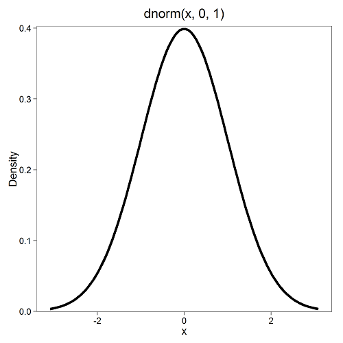
Figure 1. Density plot of standard normal distribution
Next, here’s the t-distribution for five degrees of freedom (Fig 2).
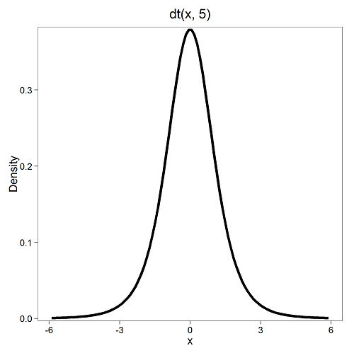
Figure 2. Density plot of t-distribution for five degrees of freedom.
Lets see what happens to the shape of the t-distribution as we increase the degrees of freedom from df = 5, 10, 20, 50, 1000, 10000 (Fig 3). The last graphic in the series is the standard normal curve again (Fig 3).
Figure 3. Animated GIF of density plot t distribution, from df = 5 to 10,000 plus standard normal curve.
By convention in the Null Hypothesis Significance Testing protocol (NHST), we compare the test statistic to a critical value. The critical value is defined as the value of the test statistic that occurs at the Type I error rate, which is typically set to 5%. We introduced logic of NHST approach in Chapter 6.9 with the chi-square distribution. Again ,this is just an introduction; we teach it now as a sort of mechanical understanding to develop. The justification for this approach to testing of statistical significance is developed in Chapter 8.
Table of Critical values of the t distribution for df 1 – 5, one tail (upper)
| df | α = 0.05 | α = 0.025 | α = 0.01 |
| 1 | 6.314 | 12.706 | 31.820 |
| 2 | 2.920 | 4.303 | 6.965 |
| 3 | 2.353 | 3.182 | 4.541 |
| 4 | 2.132 | 2.776 | 3.747 |
| 5 | 2.015 | 2.571 | 3.365 |
See Appendix 20.3 for a complete table of t-distribution.
Questions
- What happens to the shape of the t distribution as degrees of freedom are increased from 1 to 5 to 20 to 100?
Be able to answer these questions using the t table, Appendix 20.3, or using Rcmdr
- For probability α = 5%, what is the critical value of the t distribution (upper tail) for 1 degree of freedom? For 5 df? For 20 df? For 30 df?
- The value of the t test statistic is given as 12. With 3 degrees of freedom, what is the approximate probability of this value, or greater from the t distribution?
Chapter 6 contents
- Introduction
- Some preliminaries
- Ratios and proportions
- Combinations and permutations
- Types of probability
- Discrete probability distributions
- Continuous distributions
- Normal distribution and the normal deviate (Z)
- Moments
- Chi-square distribution
- t distribution
- F distribution
- References and suggested readings