19.3 — Monte Carlo methods
edits: — under construction —
Introduction
Statistical method that employ Monte Carlo methods use repeated random sampling to estimate properties of a frequency distribution. These distributions may be well-known, e.g., gamma-distribution, normal distribution, or t-distribution, or . The simulation is based on generation of a set of random numbers on the open interval (0,1) — the set of real numbers between zero and one (all numbers greater than 0 and less than 1).
If the set included 0 and 1, then it would be called a closed set, i.e., the set includes the boundary points zero and one.
Markov chain Monte Carlo (MCMC) sampling approach used to solve large scale problems. The Markov chain refers to how the sample is drawn from a specified probability distribution. It can be drawn by discrete time steps (DTMC) or by a continuous process (CTMC). The Markov process is “memoryless:” predictions of future events are derived solely from their present state — the future and past states are independent.
Gibbs sampling is a common MCMC algorithm.
ccc
R code
R’s uniform generator is runif function. Examples of the samples generated over different values (100, 1000, 10000, 100000) with output displayed as histograms (Fig. 1). Note that as sample size increases, the simulated distributions resemble more and more the uniform distribution. Use set.seed() to reproduce the same set and sequence of numbers
require(RcmdrMisc)
par(mfrow = c(2, 2))
myUniformH <- data.frame(runif(100))
with(myUniformH, Hist(runif.100., scale="frequency", ylim=c(0,20), breaks="Sturges", col="red", xlab="100 samples", ylab="Count"))
myUniform1K <- data.frame(runif(1000))
with(myUniform1K, Hist(runif.1000., scale="frequency", ylim=c(0,150), breaks="Sturges", col="green", xlab="1K samples", ylab="Count"))
myUniform10K <- data.frame(runif(10000))
with(myUniform10K, Hist(runif.10000., scale="frequency", ylim=c(0,600), breaks="Sturges", col="lightblue", xlab="10K samples", ylab="Count"))
myUniform100K <- data.frame(runif(100000))
with(myUniform100K, Hist(runif.100000., scale="frequency", ylim=c(0,5000),breaks="Sturges", col="blue", xlab="100K samples", ylab="Count"))
#reset par()
dev.off()
Yes, a nice repeating function would be more elegant code, but we move on. As a suggestion, you should create one! Use sapply() or a basic for loop.
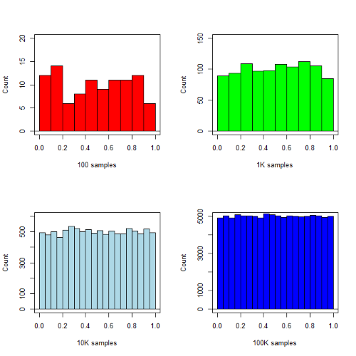
Figure 1. Histograms of runif results with 100, 1K, 10K, and 100K numbers of values to be generated
Looks pretty uniform. A property of random numbers is that history should not influence the future, i.e., no autocorrelation. We can check using the acf() function (Fig. 2).
par(mfrow = c(2, 2))
acf(myUniformH, main="100")
acf(myUniform1K, main="1K")
acf(myUniform10K, main="10K")
acf(myUniform100K, main="100K"
dev.off()
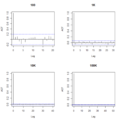
Figure 2. Autocorrelation plots of runif results with 100, 1K, 10K, and 100K numbers of values
Correlations among points are plotted versus lag, where lag refers to the number of points between adjacent points, e.g., lag = 10 reflects the correlation among points 1 and 11, 2 and 12, and so forth. The band defined by two parallel blue dashed lines
Questions
- Use
set.seed(123)and repeatrunif(10)twice. Confirm that the two sets are different (do not set seed) or the same whenset.seedis used. R hint: use functionidentical(x,y), where x and y are the two generated samples. This function tests whether the values and sequence of elements are the same between the two vectors.
Chapter 19 contents
- Introduction
- Jackknife sampling
- Bootstrap sampling
- Monte Carlo methods
- Ch19 References and suggested readings
19.2 – Bootstrap sampling
Introduction
Bootstrapping is a general approach to estimation or statistical inference that utilizes random sampling with replacement (Kulesa et al. 2015). In classic frequentist approach, a sample is drawn at random from the population and assumptions about the population distribution are made in order to conduct statistical inference. By resampling with replacement from the sample many times, the bootstrap samples can be viewed as if we drew from the population many times without invoking a theoretical distribution. A clear advantage of the bootstrap is that it allows estimation of confidence intervals without assuming a particular theoretical distribution and thus avoids the burden of repeating the experiment.
Base install of R includes the boot package. The boot package allows R users to work with most functions, and many authors have provided helpful packages. I highlight a couple packages
install packages lmboot, confintr
Example data set, Tadpoles from Chapter 14, copied to end of this page for convenience (scroll down or click here).
Bootstrapped 95% Confidence interval of population mean
Recall classic frequentist (large-sample) approach to confidence interval estimates of mean by R
x = round(mean(Tadpole$Body.mass),2); x
n = length(Tadpole$Body.mass); n
s = sd(Tadpole$Body.mass); s
error = qt(0.975,df=n-1)*(s/sqrt(n)); error
lower_ci = round(x-error,3)
upper_ci = round(x+error,3)
paste("95% CI of ", x, " between:", lower_ci, "&", upper_ci)
Output results are
> n = length(Tadpole$Body.mass); n
[1] 13
> s = sd(Tadpole$Body.mass); s
[1] 0.6366207
> error = qt(0.975,df=n-1)*(s/sqrt(n)); error
[1] 0.384706
> paste("95% CI of ", x, " between:", lower_ci, "&", upper_ci)
[1] "95% CI of 2.41 between: 2.025 & 2.795"
We used the t-distribution because both  the population mean and
  the population standard deviation were unknown. Thus, 95 out of 100 confidence intervals would be expected to include the true value.
Bootstrap equivalent
library(confintr)
ci_mean(Tadpole$Body.mass, type=c("bootstrap"), boot_type=c("stud"), R=999, probs=c(0.025, 0.975), seed=1)
Output results are
Two-sided 95% bootstrap confidence interval for the population mean based on 999 bootstrap replications
and the student method

Sample estimate: 2.412308
Confidence interval:
    2.5%    97.5%
2.075808 2.880144
where stud is short for student t distribution (another common option is the percentile method — replace stud with perc), R = 999 directs the function to resample 999 times. We set seed=1 to initialize the pseudorandom number generator so that if we run the command again, we would get the same result. Any integer number can be used. For example, I set seed = 1 for output below
Confidence interval:
    2.5%    97.5%
2.075808 2.880144
compared to repeated runs without initializing the pseudorandom number generator:
Confidence interval:
    2.5%    97.5%
2.067558 2.934055
and again
Confidence interval:
    2.5%    97.5%
2.067616 2.863158
Note that the classic confidence interval is narrower than the bootstrap estimate, in part because of the small sample size (i.e., not as accurate, does not actually achieve the nominal 95% coverage). Which to use? The sample size was small, just 13 tadpoles. Bootstrap samples were drawn from the original data set, thus it cannot make a small study more robust. The 999 samples can be thought as estimating the sampling distribution. If the assumptions of the t-distribution hold, then the classic approach would be preferred. For the Tadpole data set, Body.mass was approximately normally distributed (Anderson-Darling test = 0.21179, p-value = 0.8163). For cases where assumption of a particular distribution is unwarranted (e.g., what is the appropriate distribution when we compare medians among samples?), bootstrap may be preferred (and for small data sets, percentile bootstrap may be better). To complete the analysis, percentile bootstrap estimate of confidence interval are presented.
The R code
ci_mean(Tadpole$Body.mass, type=c("bootstrap"), boot_type=c("perc"), R=999, probs=c(0.025, 0.975), seed=1)
and the output
Two-sided 95% bootstrap confidence interval for the population mean based on 999 bootstrap replications
and the percent method
Sample estimate: 2.412308
Confidence interval:
    2.5%    97.5%
2.076923 2.749231
In this case, the bootstrap percentile confidence interval is narrower than the frequentist approach.
Model coefficients by bootstrap
R code
Enter the model, then set B, the number of samples with replacement.
myBoot <- residual.boot(VO2~Body.mass, B = 1000, data = Tadpoles)
R returns two values:
bootEstParam, which are the bootstrap parameter estimates. Each column in the matrix lists the values for a coefficient. For this model,bootEstParam$[,1]is the intercept andbootEstParam$[,2]is the slope.origEstParam, a vector with the original parameter estimates for the model coefficients.seed, numerical value for the seed; use seed number to get reproducible results. If you don’t specify the seed, then seed is set to pick any random number.
While you can list the $bootEstParam, not advisable because it will be a list of 1000 numbers (the value set with B)!
Get necessary statistics and plots
#95% CI slope
quantile(myBoot$bootEstParam[,2], probs=c(.025, .975))
R returns
    2.5%    97.5%
335.0000 562.6228
#95% CI intercept
quantile(myBoot$bootEstParam[,1], probs=c(.025, .975))
R returns
     2.5%     97.5%
-881.3893 -310.8209
Slope
#plot the sampling distribution of the slope coefficient
par(mar=c(5,5,5,5)) #setting margins to my preferred values
hist(myBoot$bootEstParam[,2], col="blue", main="Bootstrap Sampling Distribution",
xlab="Slope Estimate")
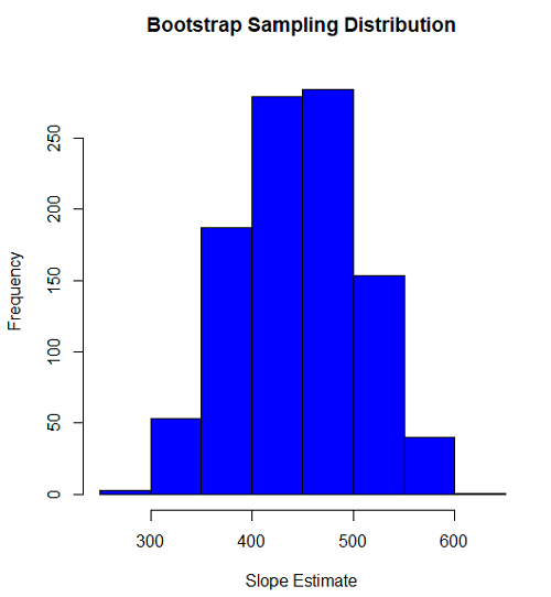
Figure 1. histogram of bootstrap estimates for slope
Intercept
#95% CI intercept
quantile(myBoot$bootEstParam[,1], probs=c(.025, .975))
par(mar=c(5,5,5,5))
hist(myBoot$bootEstParam[,1], col="blue", main="Bootstrap Sampling Distribution",
xlab="Intercept Estimate")
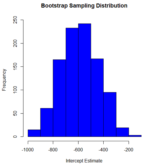
Figure 2. Histogram of bootstrap estimates for intercept.
Questions
edits: pending
Data set used this page (sorted)
| Gosner | Body mass | VO2 |
| I | 1.76 | 109.41 |
| I | 1.88 | 329.06 |
| I | 1.95 | 82.35 |
| I | 2.13 | 198 |
| I | 2.26 | 607.7 |
| II | 2.28 | 362.71 |
| II | 2.35 | 556.6 |
| II | 2.62 | 612.93 |
| II | 2.77 | 514.02 |
| II | 2.97 | 961.01 |
| II | 3.14 | 892.41 |
| II | 3.79 | 976.97 |
| NA | 1.46 | 170.91 |
Chapter 19 contents
- Introduction
- Jackknife sampling
- Bootstrap sampling
- Monte Carlo methods
- Ch19 References and suggested readings
16.1 – Product moment correlation
Introduction
A correlation is used to describe the direction  magnitude of linear association and the between two variables. There are many types of correlations, some are based on ranks, but the one most commonly used is the product-moment correlation (r). The Pearson product-moment correlation is used to describe association between continuous, ratio-scale data, where “Pearson” is in honor of Karl Pearson (b. 1857 – d. 1936).
There are many other correlations, including Spearman’s and Kendall’s tau (τ) (Chapter 16.4) and ICC, the intraclass correlation (Chapter 12.3 and Chapter 16.4).
The product moment correlation is appropriate for variables of the same kind — for example, two measures of size, like the correlation between body weight and brain weight.
Spearman’s and Kendall’s tau correlation are nonparametric and would be alternatives to the product moment correlation. The intraclass correlation, or ICC, is a parametric estimate suitable for repeat measures of the same variable.
The correlation coefficient

The numerator is the sum of products and it quantifies how the deviates from X and Y means covary together, or change together. The numerator is known as a “covariance.”

The denominator includes the standard deviations of X and Y; thus, the correlation coefficient is the standardized covariance.
The product moment correlation, r, is an estimate of the population correlation, ρ (pronounced rho), the true relationship between the two variables.

where COV(X,Y) refers to the covariance between X and Y.
Effect size
Estimates for r range from -1 to +1; the correlation coefficient has no units. A value of 0 describes the case of no statistical correlation, i.e., no linear association between the two variables. Usually, this is taken as the null hypothesis for correlation — “No correlation between two variables,” with the alternative hypothesis (2-tailed) — “There is a correlation between two variables.”
Like mean difference effect size, we can report the strength of correlation between two variables. Consider the magnitude and not the direction . Like Cohen’s effect size:
| Absolute value | Magnitude of association |
| 0.10 | small, weak |
| 0.30 | moderate |
| > 0.50 | strong, large |
Note that one should not interpret a “strong, large” correlation as evidence that the association is necessarily real. See Ch16.c for more on spurious correlations.
Standard error of the correlation
An approximate standard error for r can be obtained using this simple formula

This standard error can be used for significance testing with the t-test. See below.
Confidence interval
Like all situations in which an estimate is made, you should report the confidence interval for r. The standard error approximation is appropriate when the hull hypothesis is  , because the joint distribution is approximately normal. However, as the estimate approaches the limits of the closed interval
  , the distribution becomes increasingly skewed.
The approximate confidence interval for the correlation is based on Fisher’s z-transformation. We use this transformation to stabilize the variance over the range of possible values of the correlation and, therefore, better meet the assumptions of parametric tests based on the normal distribution.
The transform is given by the equation

where ln is the natural logarithm. In the R language we get the natural log by log(x), where x is a variable we wish to transform.
Equivalently, z can be rewritten as

the inverse hyperbolic tangent function. In R language this function is called by atanh(r) at the R prompt.
The standard error for z is about

We take z to be the estimate of the population zeta, ζ. We take the sampling distribution of z to be approximately normal and thus we may then use the normal table to generate the 95% confidence interval for zeta.

Why 1.96? We want 95% confidence interval, so that at Type I α = 0.05, we want the two tails of the Normal distribution (see Appendix 20.1), or + 0.025. Thus +0.025 is +1.96 and -1.96 corresponds to 0.025 (α = 0.05/2 tails = 0.025).
Significance testing
Significance testing of correlations is straightforward, with the noted caveat about the need to transform in cases where the estimate is close to  . For the typical test of null hypothesis, the correlation, r, is equal to 0, the t distribution can be used (i.e., it’s a t-test).

which has degrees of freedom, DF = n – 2.
Use the t-table critical values to test the null hypothesis involving product moment correlation (e.g., Appendix 20.3; for Spearman rank correlation  , see Table G, p. 686 in Whitlock & Schluter).
Alternatively (and preferred), we’ll just use R and Rcmdr’s facilities without explanation; the t distribution works OK as long as the correlations are not close to , in which case other things need to be done — and this is also true if you want to calculate a confidence interval for the correlation.
You are sufficiently skilled at this point to evaluate whether a correlation is statistically significantly different from zero — just check out whether the associated P-value is less than or greater than alpha (usually set at 5%). A test of whether or not the correlation, r1, is equal to some value, r2, other than zero is also possible. For an approximate test, replace zero in the above test statistic calculation with the value for r2, and calculate the standard error of the difference. Note that use of the t-test for significance testing of the correlation is an approximate test — if the correlations are small in magnitude using the Fisher’s Z transformation approach will be less biased, where the test statistic z now is

and standard error of the difference is

and look up the critical value of z from the normal table.
R code
To calculate correlations in R and Rcmdr, have ratio-scale data ready in the columns of a R and Rcmdr data frame. We’ll introduce the commands with an example data set from my genetics laboratory course.
Question. What is the estimate of the product moment correlation between Drosophila fly wing length and area?
Data (thanks to some of my genetics students!)
Area <- c(0.446, 0.876, 0.390, 0.510, 0.736, 0.453, 0.882, 0.394, 0.503, 0.535, 0.441, 0.889, 0.391, 0.514, 0.546, 0.453, 0.882, 0.394, 0.503, 0.535)
Length <- c(1.524, 2.202, 1.520, 1.620, 1.710, 1.551, 2.228, 1.460, 1.659, 1.719, 1.534, 2.223, 1.490, 1.633, 1.704, 1.551, 2.228, 1.468, 1.659, 1.719)
Create your data frame, e.g.,
FlyWings <- data.frame(Area, Length)
And here’s the scatterplot (Fig. 1). We can clearly see that Wing Length and Wing Area are positively correlated, with one outlier (Fig. 1).
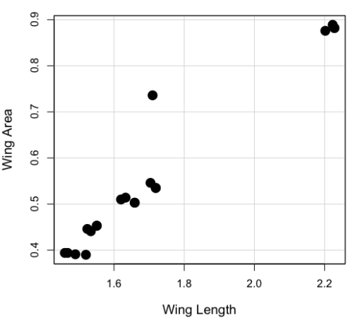
Figure 1. Scatterplot of Drosophila wing area by wing length
The R command for correlation is simply cor(x,y). This gives the “pearson” product moment correlation, the default. To specify other correlations, use method = "kendall", or method = "spearman" (See Chapter 16.4).
Question. What are the Pearson, Spearman, and Kendall’s tau estimates for the correlation between fly Wing Length and Wing Area?
At the R prompt, type
cor(Length,Area)
[1] 0.9693334
cor(Length,Area, method="kendall")
[1] 0.8248008
cor(Length,Area, method="spearman")
[1] 0.9558658
Note that we entered Length first. On your own, confirm that the order of entry does not change the correlation estimate. To both estimate test the significance of the correlation between Wing Area and Wing Length, at the R prompt type
cor.test(Area, Length, alternative="two.sided", method="pearson")
R returns with
Pearson's product-moment correlation

data: Area and Length

t = 16.735, df = 18, p-value = 2.038e-12>
alternative hypothesis: true correlation is not equal to 0
95 percent confidence interval:
0.9225336 0.9880360
sample estimates:
   cor
0.9693334
Alternatively, to calculate and test the correlation, use R Commander, Rcmdr: Statistics → Summaries→ Correlation test
R’s cor.test uses Fisher’s z transformation; note if we instead use the approximate calculation instead how poor the approximation works in this example. The estimated correlation was 0.97, thus the approximate standard error was 0.058. The confidence interval (t-distribution, alpha=0.05/2 and 18 degrees of freedom) was between 0.848 and 1.091, which is greater than the z transform result and returns an out-of-bounds upper limit.
Alternative packages to base R provide more flexibility and access to additional approaches to significance testing of correlations (Goertzen and Cribbie 2010). For example, z_cor_test() from the TOSTER package.
z_cor_test(Area, Length)

Pearson's product-moment correlation
data:  Area and Length
z = 8.5808, N = 20, p-value < 2.2e-16
alternative hypothesis: true correlation is not equal to 0
95 percent confidence interval:
0.9225336 0.9880360
sample estimates:
      cor
0.9693334
To confirm, check the critical value for z = 8.5808, two-tailed, with
> 2*pnorm(c(8.5808), mean=0, sd=1, lower.tail=FALSE)
[1] 9.421557e-18
Note the difference is that Fisher’s z is used for hypothesis testing; cor.test and z_cor_test return same confidence intervals.
and by bootstrap resampling (see Chapter 19.2),
boot_cor_test(Area, Length)

Bootstrapped Pearson's product-moment correlation

data: Area and Length
N = 20, p-value < 2.2e-16
alternative hypothesis: true correlation is not equal to 0
95 percent confidence interval:
0.8854133 0.9984744
sample estimates:
cor
0.9693334
The z-transform confidence interval would be preferred over the bootstrap confidence interval because it is narrower.
Assumptions of the product-moment correlation
Interestingly enough, there are no assumptions for estimating a statistic. You can always calculate an estimate, although of course, this does not mean that you have selected the best calculation to describe the phenomenon in question, it just means that assumptions are not applicable for estimation. Whether it is the sample mean or the correlation, it is important to appreciate that, look, you can always calculate it, even if it is not appropriate!
Statistical assumptions and those technical hypotheses we evaluate apply to statistical inference — being able to correctly interpret a test of statistical significance for a correlation estimate depends on how well assumptions are met. The most important assumption for a null hypothesis test of correlation is that samples were obtained from a “bivariate normal distribution.” It is generally sufficient to just test normality of the variables one at a time (univariate normality), but the student should be aware that testing the bivariate normality assumption can be done directly (e.g., Doornick and Hansen 2008).
Testing two independent correlations
Extending from a null hypothesis of the correlation is equal to zero to the correlation equals a particular value should not be a stretch for you. For example, since we use the t-test to evaluate the null hypothesis that the correlation is equal to zero, you should be able to make the connection that, like the two sample t-test, we can extend the test of correlation to any value. However, using the t-test without considering the need to stabilize the variance.
When two correlations come from independent samples, we can test whether or not the two correlations are equal. Rather than use the t-test, however, we use a modification of Fisher’s Z transformation. Calculate z for each correlation separately, then use the following equation to obtain Z. We then look up Z from our table of standard normal distribution (Appendix 20.1, or better — use the normal distribution functions in Rcmdr) and we can obtain the p-value of the test of the hypothesis that the two correlations are equal.

Example. Two independent correlations are r1 = 0.2 and r2 = 0.34. Sample sizes for group 1 was 14 and for group 2 was 21. Test the hypothesis that the two correlations are equal. Using R as a calculator, here’s what we might write in the R script window and the resulting output. It doesn’t matter which correlation we set as r1 or r2, so I prefer to calculate the absolute value of Z and then get the probability from the normal table for values greater or equal to |Z| (i.e., the upper tail).
z1 = atanh(0.2)
z2 = atanh(0.34)
n1 = 14
n2 = 21
Z = abs((z1-z2)/sqrt((1/(n1-3))+(1/(n2-3))))
Z = 0.3954983
From the normal distribution table we get a p-value of 0.3462 for the upper tail. Because this p-value is not less than our typical Type I error rate of 0.05, we conclude that the two correlations are not in fact significantly different.
Rcmdr: Distributions → Continuous distributions → Normal distribution → Normal probabilities…
pnorm(c(0.3954983), mean=0, sd=1, lower.tail=FALSE)
R returns
[1] 0.3462376
To make this two-tailed, of course all we have to do is multiple the one-tailed p-value by two, in this case two-tailed p-value = 0.69247.
Write a function in R
There’s nothing wrong with running the calculations as written. But R allows users to write their own functions. Here’s one possible function we could write to test two independent correlations. Write the R function in the script window.
test2Corr = function(r1,r2,n1,n2) {
z1=atanh(r1); z2=atanh(r2)
Z = abs((z1-z2)/sqrt((1/(n1-3))+(1/(n2-3))))
pnorm(c(Z), mean=0, sd=1, lower.tail=FALSE)
}
After submitting the function, we then invoke the function by typing at the R prompt
p = test2Corr(0.2,0.34,14,21); p
Again, R returns the one-tailed p-value
[1] 0.3462376
Unsurprisingly, these simple functions are often available in an R package. In this case, the psych package provides a function called r.test() which will accommodate the test of the equality hypothesis of two independent correlations. Assuming that the psych package has been installed, at the R prompt we type
require(psych)
r.test(14,.2,.34,n2=21,twotailed=TRUE)
And R returns
Correlation tests
Call:r.test(n = 14, r12 = 0.20, r34 = 0.34, n2 = 21, twotailed = TRUE)
Test of difference between two independent correlations
z value 0.4 with probability 0.69
More on testing correlations
The discussion above, as stated, assumes the two correlations are independent of each other. In ecological studies, for example, it is not uncommon to have estimates for correlations among multiple pairs of traits. Thus, our approach would not be appropriate for testing whether the difference in correlations between body mass/ornament size and body mass/swimming performance of male killifish because both correlations include the same variable (body mass).
Note: This example was selected from Sowersby et al 2022 — I’m not implying here that the authors analyzed their results incorrectly, I just like the example of traits to illustrate the point!
The r.test() in psyche package can be modified to handle this —
add Diedenhofen and Musch (2015)
cc
Questions
- True of False. It is relatively easy to move from the estimation of one correlation between two continuous variables, to the estimation of multiple pairwise (“2 at a time”) correlations among many variables. For k = the number of variables, there are k(k-1)/2 unique correlations. However, one should be concerned about the multiple comparisons problem as introduced in ANOVA when one tests for the statistical significance of many correlations.
- True or False. Generally, the null hypothesis of a test of a correlation is Ho: r = 0, although in practice, one could test a null of r = any value.
- Return to the fly wing example. What was the estimate of the value of the product moment correlation? The Spearman Rank correlation? The Kendall’s tau?
- OK, you have three correlation estimates for test of the same null hypothesis, i.e., correlation between Length and Area is zero. Which estimate is the best estimate?
- Apply the Fisher z transformation to the estimated correlation, what did you get?
- For the fly wing example, what were the degrees of freedom?
- For the fly wing example, calculate the approximate standard error of the product moment correlation.
- Return one last time to the fly wing example. What was the value of the lower limit of the 95% confidence interval for the estimate of the product moment correlation? And the value of the upper limit?
- Assume that another group of students (n = 15) made measurements on fly wings and the correlation was 0.86. Is the difference between the two correlations for the two groups of students equal? Obtain the probability using the Z calculation and R (Chapter 6.7) or the normal table.
Chapter 16 contents
8.6 – Confidence limits for the estimate of population mean
Introduction
In Chapter 3.4 and Chapter 8.3, we introduced the concept of providing a confidence interval for estimates. We gave a calculation for an approximate confidence interval for proportions and for the Number Needed to Treat (Chapter 7.3). Even an approximate confidence interval gives the reader a range of possible values of a population parameter from a sample of observations.
In this chapter we review and expand how to calculate the confidence interval for a sample mean,  . Because is derived from a sample of observations, we use the t-distribution to calculate the confidence interval. Note that if the population was known (population standard deviation), then you would use normal distribution. This was the basis for our recommendation to adjust your very approximate estimate of a confidence interval for an estimate by replacing the “2” with “1.96” when you multiply the standard error of the estimate (SE) in the equation estimate
  . As you can imagine, the approximation works for large sample size, but is less useful as sample size decreases.
Consider ; it is a point estimate of , the population mean (a parameter). But our estimate of is but one of an infinite number of possible estimates. The confidence interval, however, gives us a way to communicate how reliable our estimate is for the population parameter. A 95% confidence interval, for example, tells the reader that we are willing to say (95% confident) the true value of the parameter is between these two numbers (a lower limit and an upper limit). The point estimate (the sample mean) will of course be included between the two limits.
Instead of 95% confidence, we could calculate intervals for 99%. Since 99% is greater than 95%, we would communicate our certainty of our estimate.
Note 1: Again, the caveats about p-value extend to confidence intervals. See Chapter 8.2.
Question 1: For 99% confidence interval, the lower limit would be smaller than the lower limit for a 95% confidence interval.
- True

- False
When we set the Type I error rate,  (alpha) = 0.05 (5%), that means that 5% of all possible sample means from a population with mean, , will result in t values that are larger than
  OR smaller than
  .
.
Why the t-distribution?
We use the t-test because, technically, we have a limited sample size and the t-distribution is more accurate than the normal distribution for small samples. Note that as sample size increases, the t-distribution is not distinguishable from the normal distribution and we could use  (Fig. 1).
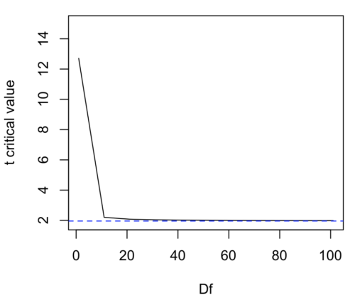
Figure 1. Critical values at Type I rate of 5% of t-distribution  . Blue dashed line is z = 1.96
Here’s the equation for calculating the confidence interval based on the t-distribution. These set the limits around our estimate of the sample mean. Together, they’re called the 95% confidence interval,  .
.
![\begin{align*} \left [ -t_{0.05\left ( 2 \right ),df} \leq \frac{\bar{X}-\mu}{s_{\bar{X}}}\leq +t_{0.05\left ( 2 \right ),df}\right ]=0.95 \end{align*}](https://biostatistics.letgen.org/wp-content/ql-cache/quicklatex.com-3d905fd4c1df0b005fb5dbd6de5fda44_l3.png "Rendered by QuickLaTeX.com")
Here’s a simplified version of the same thing, but generalized to any Type I level…

This statistic allows us to say that we are 95% confident that the interval includes the true value for . For this confidence interval you need to identify the critical t value at 5%. Thus, you need to know the degrees of freedom for this problem, which is simply  , the sample size minus one.
It is straightforward to calculate these by hand, but…
Set the Type I error rate, calculate the degrees of freedom (df):
 samples for one sample test
- pairs of samples for paired test
 samples for two independent sample test
and lookup the critical value from the t table (or from the t distribution in R). Of course, it is easier to use R.
In R, for the one tail critical value with seven degrees of freedom, type at the R prompt
qt(c(0.05), df=7, lower.tail=FALSE)
[1] 1.894579
For the two-tail critical value
qt(c(0.025), df=7, lower.tail=FALSE)
[1] 2.364624
Or, if you prefer to use R Commander, then follow the menu prompts to bring up the t quantiles function (Fig. 2 and Fig. 3)
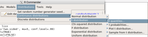
Figure 2. Drop down menu to get t-distribution
Note 2: Quantiles divide probability distribution into equal parts or intervals. Quartiles have four groups, deciles have ten groups, and percentiles have 100 groups.

Figure 3. Menu for t quantiles, with values entered for the two-tail example.
You should confirm that what R calculates agrees with the critical values tabulated in the Table of Critical values for the t distribution provided in the Appendix.
A worked example
Let’s revisit our lizard example from last time (see Chapter 8.5). Prior to conducting any inference test, we decide acceptable Type I error rates (cf. justify alpha discussion in Ch8.1); For this example, we set Type I error rate to be 1% for a 99% confidence interval.
The Rcmdr output was
t.test(lizz$bm, alternative='two.sided', mu=5, conf.level=.99)
data: lizz$bm
t = -1.5079, df = 7, p-value = 0.1753
alternative hypothesis: true mean is not equal to 5
99 percent confidence interval:
1.984737 6.199263
sample estimates:
mean of x
4.092
Sort through the output and identify what you need to know.
Question 1: What was the sample mean?
- 5
- -1.5079
- 7
- 0.1753
- 1.984737
- 6.199263
- 4.092
Question 2: What was the most likely population mean?
- 5
- Answer
- -1.5079
- 7
- 0.1753
- 1.984737
- 6.199263
- 4.092
Question 3: This was a “one-tailed” test of the null hypothesis?
- True
- False
The output states “alternative hypothesis: true mean is not equal to 5” — so it was a two-tailed test.
Question 4: What was the lower limit of the confidence interval?
- 5
- -1.5079
- 7
- 0.1753
- 1.984737
- 6.199263
- 4.092
The 99% confidence interval,  , is
, is  , which means we are 99% certain that the population mean is between
  (lower limit) and
  (upper limit). In Chapter 8.5 we calculated the , is
  .
.
Confidence intervals by nonparametric bootstrap sampling
Bootstrapping is a general approach to estimation or statistical inference that utilizes random sampling with replacement (Kulesa et al. 2015). In classic frequentist approach, a sample is drawn at random from the population and assumptions about the population distribution are made in order to conduct statistical inference. By resampling with replacement from the sample many times, the bootstrap samples can be viewed as if we drew from the population many times without invoking a theoretical distribution. A clear advantage of the bootstrap is that it allows estimation of confidence intervals without assuming a particular theoretical distribution and thus avoids the burden of repeating the experiment. Which method to prefer? For cases where assumption of a particular distribution is unwarranted (e.g., what is the appropriate distribution when we compare medians among samples?), bootstrap may be preferred (and for small data sets, percentile bootstrap may be better). We cover bootstrap sampling of confidence intervals in Chapter 19.2 Bootstrap sampling.
Conclusions
The take home message is simple.
- All estimates must be accompanied by a Confidence Interval
- The more confident we wish to be, the wider the confidence interval will be
Note that the confidence interval concept combines DESCRIPTION (the population mean is between these limits) and INFERENCE (and we are 95% certain about the values of these limits). It is good statistical practice to include estimates of confidence intervals for any estimate you share with readers. Any statistic that can be estimated should be accompanied by a confidence interval and, as you can imagine, formulas are available to do just this. For example, earlier this semester we calculated NNT.
Questions
- Note in the worked example we used Type I error rate of 1%, not 5%.
- With a Type I error rate of 5% and sample size of 10, what will be the degrees of freedom (df) for the t distribution?
- Considering the information in question 1, what will be the critical value of the t-distribution for
- a one tail test?
- a two-tail test
- To gain practice with calculations of confidence intervals, calculate the approximate confidence interval, the 95% and the 99% confidence intervals based on the t distribution, for each of the following.
-
- = 13,
 = 1.3,
  = 10
= 10 - = 13, = 1.3, = 30
- = 13, = 2.6, = 10
- = 13, = 2.6, = 30
- Take at look at your answers to question 3 — what trend(s) in the confidence interval calculations do you see with respect to variability?
- Take at look at your answers to question 3 — what trend(s) in the confidence interval calculations do you see with respect to sample size?
Chapter 8 contents
- Introduction
- The null and alternative hypotheses
- The controversy over proper hypothesis testing
- Sampling distribution and hypothesis testing
- Tails of a test
- One sample t-test
- Confidence limits for the estimate of population mean
- References and suggested readings
8.5 – One sample t-test
Introduction
We’re now talking about the traditional, classical two group comparison involving continuous data types. Thus begins your introduction to parametric statistics. One sample tests involve questions like, how many — what proportion of — people would we expect are shorter or taller than two standard deviations from the mean? This type of question assumes a population and we use properties of the normal distribution and, hence, these are called parametric tests because the assumption is that the data has been sampled from a particular probability distribution.
However, when we start asking questions about a sample statistic (e.g., the sample mean), we cannot use the normal distribution directly, i.e., we cannot use Z and the normal table as we did before (Chapter 6.7). This is because we do not know the population standard deviation and therefore must use an estimate of the variation (s) to calculate the standard error of the mean.
With the introduction of the t-statistic, we’re now into full inferential statistics-mode. What we do have are estimates of these parameters. The t-test — aka Student’s t-test — was developed for the purpose of testing sample means when the true population parameters are not known.
Note 1: It’s called Student’s t-test after the pseudonym used by William Gosset.
The equation of the one sample t-test. Note the resemblance in form with the Z-score!

where  is the sample standard error of the sample mean (SEM).
For example, weight change of mice given a hormone (leptin) or placebo. The  , but under the null hypothesis, the mean change is “really” zero (
 ). How unlikely is our value of 5 g?
Note 2: Did you catch how I snuck in “placebo” and mice? Do you think the concept of placebo is appropriate for research with mice, or should we simply refer to it as a control treatment? See Ch5.4 – Clinical trials for review.
Speaking of null hypotheses, can you say (or write) the null and alternative hypotheses in this example? How about in symbolic form?
We want to know if our sample mean could have been obtained by chance alone from a population where the true change in weight was zero.
and
and we take these values and plug them into our equation of the t-test
Then recall that Degrees of Freedom are DF = n – 1 so we have DF = 20 – 1 = 19 for the one sample t-test. And the Critical Value is found in the appropriate table of critical values for the t distribution (Fig. 1)
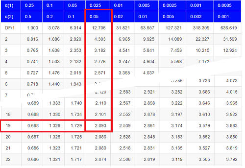
Figure 1. Table of a portion of the Critical values of the t distribution. Red selections highlight critical value for t-test at α = 5% and df = 19.
Note 3: See our table of critical values of t distribution.
Or, and better, use R
qt(c(0.025), df=19, lower.tail=FALSE)
where qt() is function call to find t-score of the pth percentile (cf 3.3 – Measures of dispersion) of the Student t distribution. For a two tailed text, we recall that 0.025 is lower tail and 0.025 is upper tail.
In this example we would be willing to reject the Null Hypothesis if there was a positive OR a negative change in weight.
This was an example of a “two-tailed test” which is “2-tail” or α(2) in Table of critical values of the t distribution.
Critical Value for α(2) = 0.05, df = 19, = 2.093
Do we accept or reject the Null Hypothesis?
A typical inference workflow
Note the general form of how the statistical test is processed, a form which actually applies to any statistical inference test.
- Identify the type of data
- State the null hypothesis (2 tailed? 1 tailed?)
- Select the test statistic (t-test) and determine its properties
- Calculate the test statistic (the value of the result of the t-test)
- Find degrees of freedom
- For the DF, get the critical value
- Compare critical value to test statistic
- Do we accept or reject the null hypothesis?
And then we ask, given the results of the test of inference, What is the biological interpretation? Statistical significance is not necessarily evidence of biological importance. In addition to statistical significance, the magnitude of the difference — the effect size — is important as part of interpreting results from an experiment. Statistical significance is at least in part because of sample size — the large the sample size, the smaller the standard error of the mean, therefore even small differences may be statistically significant, yet biologically unimportant. Effect size is discussed in Ch9.1 – Chi-square test: Goodness of fit, Ch11.4 – Two sample effect size and Ch12.5 – Effect size for ANOVA.
R Code
Let’s try a one-sample t-test. Consider the following data set: body mass of four geckos and four Anoles lizards (Dohm unpublished data).
For starters, let’s say that you have reason to believe that the true mean for all small lizards is 5 grams (g).
Geckos: 3.186, 2.427, 4.031, 1.995
Anoles: 5.515, 5.659, 6.739, 3.184
Get the data into R (Rcmdr)
By now you should be able to load this data in one of several ways. If you haven’t already entered the data, check out Part 07. Working with your own data in Mike’s Workbook for Biostatistics.
Once we have our data.frame, proceed to carry out the statistical test.
To get the one-sample t-test in Rcmdr, click on Statistics → Means → Single-sample t-test… Because there is only one numerical variable, Body.mass, that is the only one that shows up in the Variable (pick one) window (Fig 2)
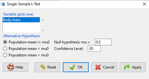
Figure 2. Screenshot Rcmdr single-sample t-test menu.
Type in the value 5.0 in the Null hypothesis =mu box.
Question 3: Quick! Can you write, in plain old English, the statistical null hypothesis???
Click OK
The results go to the Output Window.
t.test(lizards$Body.mass, alternative='two.sided', mu=5.0, conf.level=.95)
One Sample t-test
data: lizards$Body.mass
t = -1.5079, df = 7, p-value = 0.1753
alternative hypothesis: true mean is not equal to 5
95 percent confidence interval:
2.668108 5.515892
sample estimates:
mean of x 4.092
end of R output
Let’s identify the parts of the R output from the one sample t-test. R reports the name of the test and identifies
- The
dataset$variableused (lizards$Body.mass). The data set was called “lizards” and the variable was “Body.mass”. R uses the dollar sign ($) to denote the dataset and variable within the data set. - The value of the t test statistic was (t = -1.5079). It is negative because the sample mean was less than the population mean — you should be able to verify this!
- The degrees of freedom, df = 7
- The p-value = 0.1753
- 95% confidence interval of the population mean; lower limit = 2.668108, upper limit = 5.515892
- The sample mean = 4.092
Take a step back and review
Lets make sure we “get” the logic of the hypothesis testing we have just completed.
Consider the one-sample t-test.
Step 1. Define HO and HA. The null hypothesis might be that a sample mean, , is equal to μ = 5.
The alternate is that the sample mean is not equal to 20.
Where did the value 5 come from? It could be a value from the literature (does the new sample differ from values obtained in another lab?). The point is that the value is known in advance, before the experiment is conducted, and that makes it a one-sample t-test.
One tailed hypothesis or two?
We introduced you to the idea of “tails of a test” (Ch08.4). As you should recall, a null/alternate hypothesis for a two-tailed test may be written as
Null hypothesis

versus the alternative hypothesis

where is the sample mean and is the population mean.
Alternatively, we can write one-tailed tests of null/alternate hypothesis

for the null hypothesis versus the alternate hypothesis

Question 4: Are all possible outcomes of the one-tailed test covered by these two hypotheses?
Question 5: What is the SEM for this problem?
Question 6: What is the difference between a one sample t-test and a one-sided test?
Question 7: What are some other possible hypotheses that can be tested from this simple example of two lizard species?
Step 2. Decide how certain you wish to be (with what probability) that the sample mean is different from μ. As stated previously, in biology, we say that we are willing to be incorrect 5% of the time (Cowles and Davis 1982; Cohen 1994). This means we are likely to correctly reject the null hypothesis 100% – 5% = 95% of the time, which is the definition of statistical power. We do this by setting the Type I error to be 5% (alpha, α = 0.05). The Type I error is the chance that we will reject a null hypothesis, but the true condition in the population we sampled was actually “no difference.”
Step 3. Carry out the calculation of the test statistic. In other words, get the value of t from the equation above by hand, or, if using R (yes!) simply identify the test statistic value from the R output after conducting the one sample t test.
Step 4. Evaluate the result of the test. If the value of the test statistic is greater than the critical value for the test, then you conclude that the chance (the P-value) that the result could be from that population is not likely and you therefore reject the null hypothesis.
Question 8: What is the critical value for a one-sample t-test with df = 7?
Hint; you need the table or better, use R
Rcmdr: Distributions → Continuous distributions → t distributions → t quantiles
You also need to know three additional things to answer this question.
- You need to know alpha (α), which we have said generally is set at 5%.
- You also need to know the degrees of freedom (DF) for the test. For a one sample t-test, DF = n – 1, where n is the sample size.
- You also must know whether your test is one or two-tailed.
- You then use the t-distribution (the tables of the t-distribution at the back of your book) to obtain the critical value. Note that if you use R, the actual p-value is returned.
Why learn the equations when I can just do this in R?
Rcmdr does this for you as soon as you click OK. Rcmdr returns the value of the test statistic and the p-value. R does not show you the critical value, but instead returns the probability that your test statistic is as large as it is AND the null hypothesis is true. From our one-sample t-test example, the Rcmdr output. The simple answer is that in order to understand the R output properly you need to know where each item of the output for a particual test comes from and how to interpret it. Thus, the best way is to have the equations available and to understand the algorithmic approach to statistical inference.
And, this is as good of time as any to show you how to skip the RCmdr GUI and go straight to R.
First, create your variables. At the R prompt enter the first variable
liz <- c("G","G","G","G","A","A","A","A")
and then create the second variable
bm <- c(3.186,2.427,4.031,1.995,5.515,5.659,6.739,3.184)
Next, create a data frame. Think of a data frame as another word for worksheet.
lizz <- data.frame(liz,bm)
Verify that entries are correct. At the R prompt type “lizz” wthout the quotes and you should see
lizz
 liz bm
1 G 3.186
2 G 2.427
3 G 4.031
4 G 1.995
5 A 5.515
6 A 5.659
7 A 6.739
8 A 3.184
End of R output
Carry out the t-test by typing at the R prompt the following
t.test(lizz$bm, alternative='two.sided', mu=5, conf.level=.95)
And, like the Rcmdr output we have for the one-sample t-test the following R output
One Sample t-test
data: lizards$Body.mass
t = -1.5079, df = 7, p-value = 0.1753 alternative hypothesis: true mean is not equal to 5
95 percent confidence interval:
2.668108 5.515892
sample estimates:
mean of x
4.092
End of R output
which, as you probably guessed, is the same as what we got from RCmdr.
Question 9: From the R output of the one sample t-test, what was the value of the test statistic?
- -1.5079
- 7
- 0.1753
- 2.668108
- 5.515892
- 4.092
Note. On an exam you will be given portions of statistical tables and output from R. Thus you should be able to evaluate statistical inference questions by completing the missing information. For example, if I give you a test statistic value, whether the test is one- or two-tailed, degrees of freedom, and the Type I error rate alpha, you should know that you would need to find the critical value from the appropriate statistical table. On the other hand, if I give you R output, you should know that the p-value and whether it is less than the Type I error rate of alpha would be all that you need to answer the question.
Think of this as a basic skill.
In statistics and for some statistical tests, Rcmdr and other software may not provide the information needed to decide that your test statistic is large, and a table in a statistics book is the best way to evaluate the test.
For now, double check Rcmdr by looking up the critical value from the t-table.
Check critical value against our test statistic
Df = 8 – 1 = 7
The test is two-tailed, therefore α(2)
α = 0.05 (note that two-tailed critical value is 2.365. T was equal to 1.51 (since t-distribution is symmetrical, we can ignore the negative sign), which is smaller than 2.365 and so we would agree with Rcmdr — we cannot reject the null hypothesis.
Question 10: From the R output of the one sample t-test, what was the P-value?
- -1.5079
- 7
- 0.1753
- 2.668108
- 5.515892
Question 10: We would reject the null hypothesis
- False
- True
Questions
Eleven questions were provided for you within the text in this chapter. Here’s one more.
12. Here’s a small data set for you to try your hand at the one-sample t-test and Rcmdr. The dataset contains cell counts, five counts of the numbers of beads in a liquid with an automated cell counter (Scepter, Millipore USA). The true value is 200,000 beads per milliliter fluid; the manufacturer claims that the Scepter is accurate within 15%. Does the data conform to the expectations of the manufacturer? Write a hypothesis then test your hypothesis with the one-sample t-test. Here’s the data.
| scepter |
| 258900 |
| 230300 |
| 107700 |
| 152000 |
| 136400 |
Chapter 8 contents
8.4 – Tails of a test
Introduction
The basics of statistical inference is to establish the null and alternative hypotheses. Starting with the simplest cases, where there is one sample of observations and the comparison is against a population (theory) mean, how many possible comparisons can be made? The next simplest is the two-sample case, where we have two sets of observations and the comparison is against the two groups. Again, how many total comparisons may be made?
Let , “X bar”, equal the sample mean and , “mu”, represent the population mean. For sample means, designate groups by a subscript, 1 or 2. We then have Table 1.
Table 1. Possible hypothesis involving two groups
| Comparison | One-same | Two-sample |
| 1. |  |
 |
| 2. |  |
 |
| 3. |  |
 |
| 4. |  |
 |
| 5. |  |
 |
| 6. |  |
 |
Classical statistics classifies inference into null hypothesis, HO, vs. alternate hypotheses, HA, and specifies that we test null hypotheses based on the value of the estimated test statistic (see discussion about critical value and p-value, Chapter 8.2). From the list of six possible comparisons we can divide them into one-tailed and two-tailed differences (Table 1). By “tail” we are referring to the ends or tails of a distribution (Figure 1, Figure 2); where do our results fall on the distribution?
Two-tailed hypotheses: Comparison 1 and comparison 2 in the table above are two-tailed hypotheses. We don’t ask about the direction of any difference (less than or greater than).
Figure 1 shows the “two-tailed” distribution — if our results fall to the left ,  , or to the right
  we reject the null hypothesis (blue regions in the curve). We divide the type I error into two equal halves.
Note. It’s a nice trick to shade in regions of the curve. A package tigerstats includes the function pnormGC that simplifies this task.
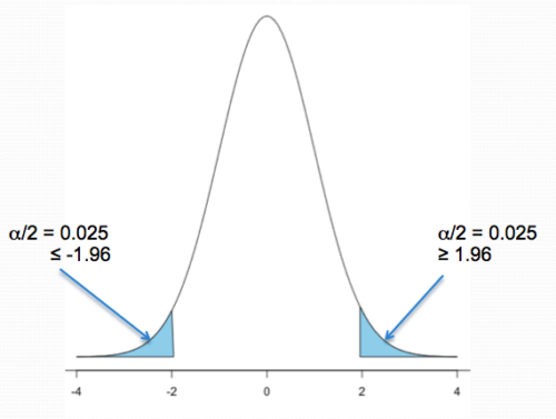
Figure 1. Two-tailed distribution.
library(tigerstats)
pnormGC(c(-1.96,1.96), region="outside", mean=0, sd=1,graph=TRUE)
Figure 2 shows the “one-tailed” distribution — if our alternate hypothesis was that the sample mean was less than the population mean, then our fall to the left,  , for the “lower tail” of the distribution. If, however, our alternate hypothesis was that the sample mean was greater than the population mean, then our region of interest falls to the right,
  . Again, we reject the null hypothesis (blue regions in the curve). Note for one-tailed hypothesis, all Type I error occurs in the one area, not both, so (alpha) remains 0.05 over the entire rejection region (Fig 2).
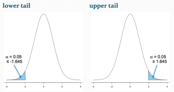
Figure 2. One-tailed distribution, lower tail (left) and upper tail (right).
library(tigerstats)
pnormGC(1.645, region="above", mean=0, sd=1,graph=TRUE)
pnormGC(-1.645, region="below", mean=0, sd=1,graph=TRUE)
One-tailed hypotheses: Comparison 3 through comparison 6 in the table are one-tailed hypotheses. The direction of the difference matters.
Note a simple trick to writing one-tailed hypotheses: first write the alternate hypothesis because the null hypothesis includes all of the other possible outcomes of the test.
Examples
Lets consider some examples. We learn best by working through cases.
Chemotherapy as an approach to treat cancers owes its origins to the work of Dr Sidney Farber among others in the 1930s and ’40s (DeVita and Chu 2008; Mukherjee 2011). Following up on the observations of others that folic acid (vitamin B9) improved anemia, Dr Farber believed that folic acid might reverse the course of leukemia (Mukherjee 2011). In 1946 he recruited several children with acute lymphoblastic leukemia and injected them with folic acid. Instead of ameliorating their symptoms (e.g., white blood cell counts and percentage of abnormal immature white blood cells, called blast cells), treatments accelerated progression of the disease. That’s a scientific euphemism for the reality — the children died sooner in Dr. Faber’s trial than patients not enrolled in his study. He stopped the trials. Clearly, adding folic acid was not a treatment against this leukemia.
Question 1. Do you think these experiments are one sample or two sample? Hint: Is there mention of a control group?
Answer: There’s no mention of a control group, but instead, Dr. Faber would have had plenty of information about the progression of this disease in children. This was a one sample test.
Question 2. What would be a reasonable interpretation of Dr Faber’s alternate hypothesis with respect to percentage of blast cells in patients given folic acid treatment? Your options are
- Folic acid supplementation has an effect on blast counts.
- Folic acid supplementation reduces blast counts.
- Folic acid supplementation increases blast counts.
- Folic acid supplementation has no effect on blast counts.
Answer: At the start of the trials, it is pretty clear that the alternate hypothesis was intended to be a one-tailed test (option 2). Dr. Faber’s alternative hypothesis clearly was that he believed that addition of folic acid would reduce blast cell counts. However, that they stopped the trials shows that they recognized that the converse had occurred, that blast counts increased; this means that, from a statistician’s point of view, Dr Faber’s team was testing a two-sided hypothesis (option 1).
Another example.
Dr Farber reasoned that if folic acid accelerated leukemia progression, perhaps anti-folic compounds might inhibit leukemia progression. Dr Farber’s team recruited patients with acute lymphoblastic leukemia and injected them with a folic acid agonist called aminopterin. Again, he predicted that blast counts would reduce following administration of the chemical. This time, and for the first time in recorded medicine, blast counts of many patients drastically reduced to normal levels and the patients experienced remissions. The remissions were not long lasting and all patients eventually succumbed to leukemia. Nevertheless, these were landmark findings — for the first time a chemical treatment was shown to significantly reduce blast cell counts, even leading to remission, if however brief (Mukherjee 2011).
Try Question 3 and Question 4 yourself.
Question 3. Do you think these experiments are one sample or two sample? Hint: Is there mention of a control group?
Question 4. What would be a reasonable interpretation of Dr Faber’s alternate hypothesis with respect to percentage of blast cells in patients given aminopterin treatment? Your options are
- Aminopterin supplementation has an effect on blast counts.
- Aminopterin supplementation reduces blast counts.
- Aminopterin supplementation increases blast counts.
- Aminopterin supplementation has no effect on blast counts.
Pros and Cons to One-sided testing
Here’s something to consider: why not restrict yourself to one-tailed hypotheses? Here’s the pro-argument. Strictly speaking you gain statistical power to test the null hypothesis. For example, look up the t-test distribution for degrees of freedom equal to 20 and compare  (one tail) vs.
  (two-tail). You will find that for the one-tailed test, the critical value of the t-distribution with 20 df is 1.725, whereas for the two-tailed test, the critical value of the t-distribution with the same numbers of df is 2.086. Thus, the difference between means can be much smaller in the one-tailed test and prove to be “statistically significant.” Put simply, with the same data, we will reject the Null Hypothesis more often with one-tailed tests.
The con-argument. If you use a one-tailed test you MUST CLEARLY justify its use and be aware that a deviation in the opposite direction MUST be ignored! More specifically, you interpret a one-tailed result in the opposite direction as acceptance of the null — you cannot, after the fact, change your mind and start speaking about “statistically significant differences” if you had specified a one-tailed hypothesis and the results showed differences in the opposite direction.
Note. Recall also that, by itself, statistical significance judged by the p-value against a specified cut-off critical value is not enough to say there is evidence for or against the hypothesis. For that we need to consider effect size, see Power analysis in Chapter 11.
Questions
- For a Type I error rate of 5% and the following degrees of freedom, compare the critical values for one tail test and a two tailed test of the null hypothesis.
- 5 df
- 10 df
- 15 df
- 20 df
- 25 df
- 30 df
- Using your findings from Additional Question 1, make a scatterplot with degrees of freedom on the horizontal axis and critical values on the vertical axis. What trend do you see for the difference between one and two tailed tests as degrees of freedom increase?
- A clinical nutrition researcher wishes to test the hypothesis that a vegan diet lowers total serum cholesterol levels compared to an omnivorous diet. What kind of hypothesis should he use, one-tailed or two-tailed? Justify your choice.
- Spironolactone, introduced in 1953, is used to block aldosterone in hypertensive patients. A newer drug eplerenone, approved by the FDA in 2002, is reported to have the same benefits as spironolactone (reduced mortality, fewer hospitalization events), but with fewer side effects compared with spironolactone. Does this sentence suggest a one-tailed test or a two-tailed test?
- Write out the appropriate null and alternative hypothesis statements for the spironolactone and eplerenone scenario.
- You open up a bag of Original Skittles and count the number of green, orange, purple, red, and yellow candies in the bag. What kind of hypothesis should be used, one-tailed or two-tailed? Justify your choice.
- Verify the probability values from the table of standard normal distribution for Z equal to -1.96, -1.645, 1.645, and 1.96.