18.2 – Nonlinear regression
Introduction
The linear model is incredibly relevant in so many cases. A quick look “linear model” in PUBMED returns about 22 thousand hits; 3.7 million in Google Scholar; 3 thousand hits in ERIC database. These results compare to search of “statistics” in the same databases: 2.7 million (PUBMED), 7.8 million (Google Scholar), 61.4 thousand (ERIC). But all models are not the same.
Fit of a model to the data can be evaluated by looking at the plots of residuals (Fig. 1), where we expect to find random distribution of residuals across the range of predictor variable.
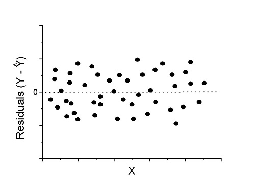
Figure 1. Ideal plot of residuals against values of X, the predictor variable, for a well-supported linear model fit to the data.
However, clearly, there are problems for which assumption of fit to line is not appropriate. We see this, again, in patterns of residuals, e.g., Figure 2.
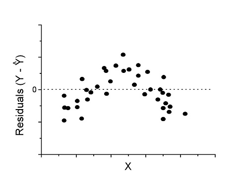
Figure 2. Example of residual plot; pattern suggests nonlinear fit.
Fitting of polynomial linear model
Fit simple linear regression
R code
LinearModel.1 <- lm(cumFreq~Months, data=yuan)

summary(LinearModel.1)

Call:
lm(formula = cumFreq ~ Months, data = yuan)

Residuals:
     Min       1Q   Median      3Q     Max
-0.11070 -0.07799 -0.01728 0.06982 0.13345

Coefficients:
                 Estimate Std. Error t value Pr(>|t|)
(Intercept)     -0.132709   0.045757   -2.90  0.0124 *
Months           0.029605   0.001854   15.97  6.37e-10 ***
---
Signif. codes: 0 '***' 0.001 '**' 0.01 '*' 0.05 '.' 0.1 ' ' 1

Residual standard error: 0.09308 on 13 degrees of freedom
Multiple R-squared: 0.9515, Adjusted R-squared: 0.9477
F-statistic: 254.9 on 1 and 13 DF, p-value: 6.374e-10
We see from the R2 (95%), a high degree of fit to the data. However, residual plot reveals obvious trend (Fig. 3)
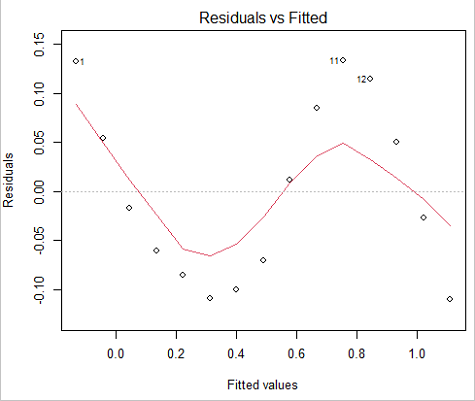
Figure 3. Residual plot
We can fit a polynomial regression.
First, a second order polynomial
LinearModel.2 <- lm(cumFreq ~ poly( Months, degree=2), data=yuan)

summary(LinearModel.2)

Call:
lm(formula = cumFreq ~ poly(Months, degree = 2), data = yuan)

Residuals:
     Min       1Q   Median      3Q     Max
-0.13996 -0.06720 -0.02338 0.07153 0.14277

Coefficients:
                           Estimate Std. Error  t value   Pr(>|t|)
(Intercept)                 0.48900    0.02458   19.891   1.49e-10 ***
poly(Months, degree = 2)1   1.48616    0.09521   15.609   2.46e-09 ***
poly(Months, degree = 2)2   0.06195    0.09521    0.651   0.528
---
Signif. codes: 0 '***' 0.001 '**' 0.01 '*' 0.05 '.' 0.1 ' ' 1

Residual standard error: 0.09521 on 12 degrees of freedom
Multiple R-squared: 0.9531, Adjusted R-squared: 0.9453
F-statistic: 122 on 2 and 12 DF, p-value: 0.0000000106
Second, try a third order polynomial
LinearModel.3 <- lm(cumFreq ~ poly(Months, degree = 3), data=yuan)

summary(LinearModel.3)

Call:
lm(formula = cumFreq ~ poly(Months, degree = 3), data = yuan)

Residuals:
      Min        1Q   Median       3Q      Max
-0.052595 -0.021533 0.001023 0.025166 0.048270

Coefficients:
                           Estimate Std. Error t value   Pr(>|t|)
(Intercept)                0.488995   0.008982  54.442   9.90e-15 ***
poly(Months, degree = 3)1  1.486157   0.034787  42.722   1.41e-13 ***
poly(Months, degree = 3)2  0.061955   0.034787   1.781   0.103
poly(Months, degree = 3)3 -0.308996   0.034787  -8.883   2.38e-06 ***
---
Signif. codes: 0 '***' 0.001 '**' 0.01 '*' 0.05 '.' 0.1 ' ' 1

Residual standard error: 0.03479 on 11 degrees of freedom
Multiple R-squared: 0.9943, Adjusted R-squared: 0.9927
F-statistic: 635.7 on 3 and 11 DF, p-value: 1.322e-12
Which model is best? We are tempted to compare R-squared among the models, but R2 turn out to be untrustworthy here. Instead, we compare using Akaike Information Criterion, AIC
R code/results
AIC(LinearModel.1,LinearModel.2, LinearModel.3)
              df       AIC
LinearModel.1  3 -24.80759
LinearModel.2  4 -23.32771
LinearModel.3  5 -52.83981
Smaller the AIC, better fit.
anova(RegModel.5,LinearModel.3, LinearModel.4)
Analysis of Variance Table

Model 1: cumFreq ~ Months
Model 2: cumFreq ~ poly(Months, degree = 2)
Model 3: cumFreq ~ poly(Months, degree = 3)
  Res.Df   RSS    Df Sum of Sq       F      Pr(>F)
1     13 0.112628
2     12 0.108789  1  0.003838  3.1719 0.1025
3     11 0.013311  1  0.095478 78.9004 0.000002383 ***
---
Signif. codes: 0 '***' 0.001 '**' 0.01 '*' 0.05 '.' 0.1 ' ' 1
Logistic regression
The Logistic regression is a classic example of nonlinear model.
R code
logisticModel <-nls(yuan$cumFreq~DD/(1+exp(-(CC+bb*yuan$Months))), start=list(DD=1,CC=0.2,bb=.5),data=yuan,trace=TRUE)
5.163059 : 1.0 0.2 0.5
2.293604 : 0.90564552 -0.07274945 0.11721201
1.109135 : 0.96341283 -0.60471162 0.05066694
0.429202 : 1.29060000 -2.09743525 0.06785993
0.3863037 : 1.10392723 -2.14457296 0.08133307
0.2848133 : 0.9785669 -2.4341333 0.1058674
0.1080423 : 0.9646295 -3.1918526 0.1462331
0.005888491 : 1.0297915 -4.3908114 0.1982491
0.004374918 : 1.0386521 -4.6096564 0.2062024
0.004370212 : 1.0384803 -4.6264657 0.2068853
0.004370201 : 1.0385065 -4.6269276 0.2068962
0.004370201 : 1.0385041 -4.6269822 0.2068989
summary(logisticModel)

Formula: yuan$cumFreq ~ DD/(1 + exp(-(CC + bb * yuan$Months)))

Parameters:
      Estimate  Std. Error  t value      Pr(>|t|)
DD    1.038504    0.014471    71.77   < 2e-16 ***
CC   -4.626982    0.175109   -26.42  5.29e-12 ***
bb    0.206899    0.008777    23.57  2.03e-11 ***
---
Signif. codes: 0 '***' 0.001 '**' 0.01 '*' 0.05 '.' 0.1 ' ' 1

Residual standard error: 0.01908 on 12 degrees of freedom

Number of iterations to convergence: 11
Achieved convergence tolerance: 0.000006909

> AIC(logisticModel)
[1] -71.54679
Logistic regression is a statistical method for modeling the dependence of a categorical (binomial) outcome variable on one or more categorical and continuous predictor variables (Bewick et al 2005).
The logistic function is used to transform a sigmoidal curve to a more or less straight line while also changing the range of the data from binary (0 to 1) to infinity (-∞,+∞). For event with probability of occurring p, the logistic function is written as

where ln refers to the natural logarithm.
This is an odds ratio. It represents the effect of the predictor variable on the chance that the event will occur.
The logistic regression model then very much resembles the same as we have seen before.

In R and Rcmdr we use the glm() function to model the logistic function. Logistic regression is used to model a binary outcome variable. What is a binary outcome variable? It is categorical! Examples include: Living or Dead; Diabetes Yes or No; Coronary artery disease Yes or No. Male or Female. One of the categories could be scored 0, the other scored 1. For example, living might be 0 and dead might be scored as 1. (By the way, for a binomial variable, the mean for the variable is simply the number of experimental units with “1” divided by the total sample size.)
With the addition of a binary response variable, we are now really close to the Generalized Linear Model. Now we can handle statistical models in which our predictor variables are either categorical or ratio scale. All of the rules of crossed, balanced, nested, blocked designs still apply because our model is still of a linear form.
We write our generalized linear model

just to distinguish it from a general linear model with the ratio-scale Y as the response variable.
Think of the logistic regression as modeling a threshold of change between the 0 and the 1 value. In another way, think of all of the processes in nature in which there is a slow increase, followed by a rapid increase once a transition point is met, only to see the rate of change slow down again. Growth is like that. We start small, stay relatively small until birth, then as we reach our early teen years, a rapid change in growth (height, weight) is typically seed (well, not in my case … at least for the height). The fitted curve I described is a logistic one (other models exist too). Where the linear regression function was used to minimize the squared residuals as the definition of the best fitting line, now we use the logistic as one possible way to describe or best fit this type of a curved relationship between an outcome and one or more predictor variables. We then set out to describe a model which captures when an event is unlikely to occur (the probability of dying is close to zero) AND to also describe when the event is highly likely to occur (the probability is close to one).
A simple way to view this is to think of time being the predictor (X) variable and risk of dying. If we’re talking about the lifetime of a mouse (lifespan typically about 18-36 months), then the risk of dying at one months is very low, and remains low through adulthood until the mouse begins the aging process. Here’s what the plot might look like, with the probability of dying at age X on the Y axis (probability = 0 to 1) (Fig. 4).
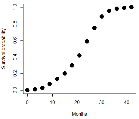
Figure 4. Lifespan of 1881 mice from 31 inbred strains (Data from Yuan et al (2012) available at https://phenome.jax.org/projects/Yuan2).
We ask — of all the possible models we could draw, which best fits the data? The curve fitting process is called the logistic regression.
With some minor, but important differences, running the logistic regression is the same as what you have been doing so far for ANOVA and for linear regression. In Rcmdr, access the logistic regression function by invoking the Generalized Linear Model (Fig. 5).
Rcmdr: Statistics → Fit models → Generalized linear model.
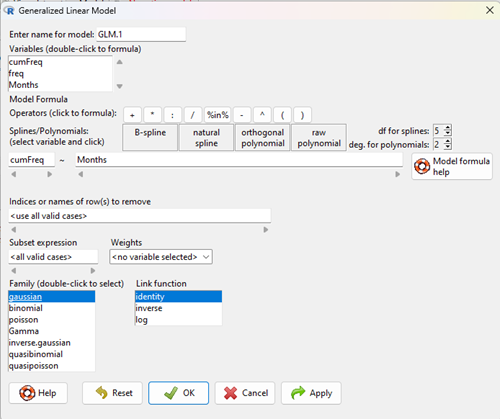
Figure 5. Screenshot Rcmdr GLM menu. For logistic on ratio-scale dependent variable, select gaussian family and identity link function.
Select the model as before. The box to the left accepts your binomial dependent variable; the box at right accepts your factors, your interactions, and your covariates. It permits you to inform R how to handle the factors: Crossed? Just enter the factors and follow each with a plus. If fully crossed, then the interactions may be specified with “:” to explicitly call for a two-way interaction between two (A:B) or a three-way interaction between three (A:B:C) variables. In the later case, if all of the two way interactions are of interest, simply typing A*B*C would have done it. If nested, then use %in% to specify the nesting factor.
R output
> GLM.1 <- glm(cumFreq ~ Months, family=gaussian(identity), data=yuan)

> summary(GLM.1)

Call:
glm(formula = cumFreq ~ Months, family = gaussian(identity),
data = yuan)

Deviance Residuals:
Min 1Q Median 3Q Max
-0.11070 -0.07799 -0.01728 0.06982 0.13345

Coefficients:
Estimate Std. Error t value Pr(>|t|)
(Intercept) -0.132709 0.045757 -2.90 0.0124 *
Months 0.029605 0.001854 15.97 6.37e-10 ***
---
Signif. codes: 0 '***' 0.001 '**' 0.01 '*' 0.05 '.' 0.1 ' ' 1

(Dispersion parameter for gaussian family taken to be 0.008663679)

Null deviance: 2.32129 on 14 degrees of freedom
Residual deviance: 0.11263 on 13 degrees of freedom
AIC: -24.808

Number of Fisher Scoring iterations: 2
Assessing fit of the logistic regression model
Some of the differences you will see with the logistic regression is the term deviance. Deviance in statistics simply means compare one model to another and calculate some test statistic we’ll call “the deviance.” We then evaluate the size of the deviance like a chi-square goodness of fit. If the model fits the data poorly (residuals large relative to the predicted curve), then the deviance will be small and the probability will also be high — the model explains little of the data variation. On the other hand, if the deviance is large, then the probability will be small — the model explains the data, and the probability associated with the deviance will be small (significantly so? You guessed it! P < 0.05).
The Wald test statistic

where n and β refers to any of the n coefficient from the logistic regression equation and SE refers to the standard error if the coefficient. The Wald test is used to test the statistical significance of the coefficients. It is distributed approximately as a chi-squared probability distribution with one degree of freedom. The Wald test is reasonable, but has been found to give values that are not possible for the parameter (e.g., negative probability).
Likelihood ratio tests are generally preferred over the Wald test. For a coefficient, the likelihood test is written as
![]()
where L0 is the likelihood of the data when the coefficient is removed from the model (i.e., set to zero value), whereas L1 is the likelihood of the data when the coefficient is the estimated value of the coefficient. It is also distributed approximately as a chi-squared probability distribution with one degree of freedom.
Questions
[pending]
Data set
| Months | freq | cumFreq |
| 0 | 0 | 0 |
| 3 | 0.01063264221159 | 0.01063264221159 |
| 6 | 0.017012227538543 | 0.027644869750133 |
| 9 | 0.045188729399256 | 0.072833599149389 |
| 12 | 0.064327485380117 | 0.137161084529506 |
| 15 | 0.064859117490697 | 0.202020202020202 |
| 18 | 0.097820308346624 | 0.299840510366826 |
| 21 | 0.118553960659224 | 0.41839447102605 |
| 24 | 0.171185539606592 | 0.589580010632642 |
| 27 | 0.162147793726741 | 0.751727804359383 |
| 30 | 0.137161084529506 | 0.888888888888889 |
| 33 | 0.069643806485912 | 0.958532695374801 |
| 36 | 0.024455077086656 | 0.982987772461457 |
| 39 | 0.011695906432749 | 0.994683678894205 |
| 42 | 0.005316321105795 | 1 |
Chapter 18 content
17.7 – Regression model fit
Introduction
In Chapter 17.5 and 17.6 we introduced the example of tadpoles body size and oxygen consumption. We ran a simple linear regression, with the following output from R
RegModel.1 <- lm(VO2~Body.mass, data=example.Tadpole)

summary(RegModel.1)

Call:
lm(formula = VO2 ~ Body.mass, data = example.Tadpole)

Residuals:
    Min      1Q    Median       3Q       Max
-202.26 -126.35     30.20    94.01    222.55

Coefficients:
                Estimate     Std. Error    t value    Pr(>|t|)
(Intercept)      -583.05         163.97     -3.556     0.00451 **
Body.mass         444.95          65.89      6.753   0.0000314 ***
---
Signif. codes: 0 '***' 0.001 '**' 0.01 '*' 0.05 '.' 0.1 ' ' 1

Residual standard error: 145.3 on 11 degrees of freedom
Multiple R-squared: 0.8057, Adjusted R-squared: 0.788
F-statistic: 45.61 on 1 and 11 DF, p-value: 0.00003144
You should be able to pick out the estimates of slope and intercept from the table (intercept was -583 and slope was 445). Additionally, as part of your interpretation of the model, you should be able to report how much variation in VO2 was explained by tadpole body mass (coefficient of determination, R2, was 0.81, which means about 81% of variation in oxygen consumption by tadpoles is explained by knowing the body mass of the tadpole.
What’s left to do? We need to evaluate how well our model fits the data, i.e., we evaluate regression model fit. By fit we mean, how well does our model agree to the raw data? A poor fit and the model predictions are far from the raw data; a good fit, the model accurately predicts the raw data. In other words, if we draw a line through the raw data, a good fit line crosses through most of the points — a poor fit the line rarely passes through the cloud of points.
How to judge fit? This we can do by evaluating the error components relative to the portion of the model that explains the data. Additionally, we can perform a number of diagnostics of the model relative to the assumptions we made to perform linear regression. These diagnostics form the subject of Chapter 17.8. Here, we ask how well does the model,

fit the data?
Model fit statistics
The second part of fitting a model is to report how well the model fits the data. The next sections apply to this aspect of model fitting. The first area to focus on is the magnitude of the residuals: the greater the spread of residuals, the less well a fitted line explains the data.
In addition to the output from lm() function, which focuses on the coefficients, we typically generate the ANOVA table also.
Anova(RegModel.1, type="II")
Anova Table (Type II tests)

Response: VO2
                Sum Sq   Df    F value       Pr(>F)
Body.mass       962870    1     45.605   0.00003144 ***
Residuals       232245   11
---
Signif. codes: 0 '***' 0.001 '**' 0.01 '*' 0.05 '.' 0.1 ' ' 1
Standard error of regression
S, the Residual Standard Error (aka Standard error of regression), is an overall measure to indicate the accuracy of the fitted line: it tells us how good the regression is in predicting the dependence of response variable on the independent variable. A large value for S indicates a poor fit. One equation for S is given by

In the above example, S = 145.3 (underlined, bold in regression output above). We can see how if SSresidual is large, S will be large indicating poor fit of the linear model to the data. However, by itself S is not of much value as a diagnostic as it is difficult to know what to make of 145.3, for example. Is this a large value for S? Is it small? We don’t have any context to judge S, so additional diagnostics have been developed.
Coefficient of determination
R2, the coefficient of determination, is also used to describe model fit. R 2, the square of the simple product moment correlation r, can take on values between 0 and 1 (0% to 100%). A good model fit has a high R 2 value. In our example above, R 2 = 0.8057 or 80.57%. One equation for R 2 is given by

A value of R 2 close to 1 means that the regression “explains” nearly all of the variation in the response variable, and would indicate the model is a good fit to the data. Note that the coefficient of determination, R 2, is the squared value of r, the product moment correlation.
Adjusted R-squared
Before moving on we need to remark on the difference between R 2 and adjusted R 2. For Simple Linear Regression there is but one predictor variable, X; for multiple regression there can be many additional predictor variables. Without some correction, R 2 will increase with each additional predictor variables. This doesn’t mean the model is more useful, however, and in particular, one cannot compare R 2 between models with different numbers of predictors. Therefore, an adjustment is used so that the coefficient of determination remains a useful way to assess how reliable a model is and to permit comparisons of models. Thus, we have the Adjusted  , which is calculated as

In our example above, Adjusted R 2 = 0.3806 or 38.06%.
Which should you report? Adjusted R2, because it is independent of the number of parameters in the model.
Both and S are useful for regression diagnostics, a topic which we will discuss next (Chapter 17.8).
Questions
- True or False. The simple linear regression is called a “best fit” line because it maximizes the squared deviations for the difference between observed and predicted Y values.
- True or False. Residuals in regression analysis are best viewed as errors committed by the researcher. If the experiment was designed better, or if the instrument was properly calibrated, then residuals would be reduced. Explain your choice.
- The USA is finishing the 2020 census as I write this note. As you know, the census is used to reapportion congress and also to determine the number of electoral college votes. In honor of the election for US President that’s just days away, in the next series of questions in this Chapter and subsequent sections of Chapter 17 and 18, I’ll ask you to conduct a regression analysis on the electoral college. For starters, make the regression of Electoral votes on 2010 census population. (Ignore for now the other columns, just focus on POP_2019 and Electoral.) Report the
- regression coefficients (slope, intercept)
- percent of the variation in electoral college votes explained by the regression (R2).
- Make a scatterplot and add the regression line to the plot
Data set
USA population year 2010 and year 2019 with Electoral College counts
| State | Region | Division | POP_2010 | POP_2019 | Electoral |
|---|---|---|---|---|---|
| Alabama | South | East South Central | 4779736 | 4903185 | 9 |
| Alaska | West | Pacific | 710231 | 731545 | 3 |
| Arizona | West | Mountain | 6392017 | 7278717 | 11 |
| Arkansas | South | West South Central | 2915918 | 3017804 | 6 |
| California | West | Pacific | 37253956 | 39512223 | 55 |
| Colorado | West | Mountain | 5029196 | 5758736 | 9 |
| Connecticut | Northeast | New England | 3574097 | 3565287 | 7 |
| Delaware | South | South Atlantic | 897934 | 982895 | 3 |
| District of Columbia | South | South Atlantic | 601723 | 705749 | 3 |
| Florida | South | South Atlantic | 18801310 | 21477737 | 29 |
| Georgia | South | South Atlantic | 9687653 | 10617423 | 16 |
| Hawaii | West | Pacific | 1360301 | 1415872 | 4 |
| Idaho | West | Mountain | 1567582 | 1787065 | 4 |
| Illinois | Midwest | East North Central | 12830632 | 12671821 | 20 |
| Indiana | Midwest | East North Central | 6483802 | 6732219 | 11 |
| Iowa | Midwest | West North Central | 3046355 | 3155070 | 6 |
| Kansas | Midwest | West North Central | 2853118 | 2913314 | 6 |
| Kentucky | South | East South Central | 4339367 | 4467673 | 8 |
| Louisiana | South | West South Central | 4533372 | 4648794 | 8 |
| Maine | Northeast | New England | 1328361 | 1344212 | 4 |
| Maryland | South | South Atlantic | 5773552 | 6045680 | 10 |
| Massachusetts | Northeast | New England | 6547629 | 6892503 | 11 |
| Michigan | Midwest | East North Central | 9883640 | 9883635 | 16 |
| Minnesota | Midwest | West North Central | 5303925 | 5639632 | 10 |
| Mississippi | South | East South Central | 2967297 | 2976149 | 6 |
| Missouri | Midwest | West North Central | 5988927 | 6137428 | 10 |
| Montana | West | Mountain | 989415 | 1068778 | 3 |
| Nebraska | Midwest | West North Central | 1826341 | 1934408 | 5 |
| Nevada | West | Mountain | 2700551 | 3080156 | 6 |
| New Hampshire | Northeast | New England | 1316470 | 1359711 | 4 |
| New Jersey | Northeast | Mid-Atlantic | 8791894 | 8882190 | 14 |
| New Mexico | West | Mountain | 2059179 | 2096829 | 5 |
| New York | Northeast | Mid-Atlantic | 19378102 | 19453561 | 29 |
| North Carolina | South | South Atlantic | 9535483 | 10488084 | 15 |
| North Dakota | Midwest | West North Central | 672591 | 762062 | 3 |
| Ohio | Midwest | East North Central | 11536504 | 11689100 | 18 |
| Oklahoma | South | West South Central | 3751351 | 3956971 | 7 |
| Oregon | West | Pacific | 3831074 | 4217737 | 7 |
| Pennsylvania | Northeast | Mid-Atlantic | 12702379 | 12801989 | 20 |
| Rhode Island | Northeast | New-England | 1052567 | 1059361 | 4 |
| South Carolina | South | South-Atlantic | 4625364 | 5148714 | 9 |
| South Dakota | Midwest | West-North-Central | 814180 | 884659 | 3 |
| Tennessee | South | East-South-Central | 6346105 | 6829174 | 11 |
| Texas | South | West-South-Central | 25145561 | 28995881 | 38 |
| Utah | West | Mountain | 2763885 | 3205958 | 6 |
| Vermont | Northeast | New-England | 625741 | 623989 | 3 |
| Virginia | South | South-Atlantic | 8001024 | 8535519 | 13 |
| Washington | West | Pacific | 6724540 | 7614893 | 12 |
| West Virginia | South | South-Atlantic | 1852994 | 1792147 | 5 |
| Wisconsin | Midwest | East-North-Central | 5686986 | 5822434 | 10 |
| Wyoming | West | Mountain | 563626 | 578759 | 3 |
Chapter 17 contents
- Introduction
- Simple Linear Regression
- Relationship between the slope and the correlation
- Estimation of linear regression coefficients
- OLS, RMA, and smoothing functions
- Testing regression coefficients
- ANCOVA – Analysis of covariance
- Regression model fit
- Assumptions and model diagnostics for Simple Linear Regression
- References and suggested readings (Ch17 & 18)
12.7 – Many tests one model
Introduction
In our introduction to parametric tests we so far have covered one and two sample t-tests and now the multiple sample or one-way analysis of variance (ANOVA). In subsequent sections we will cover additional tests, each with their own name. It is time to let you in on a little secret. All of these tests, t-tests, ANOVA, and linear and multiple regression we will work on later in the book belong to one family of statistical models. That model is called the general Linear Model (LM), not to be confused with the Generalized Linear Model (GLM) (Burton et al 1998; Guisan et al 2002). This greatly simplifies our approach to learning how to implement statistical tests in R (or other statistical programs) — you only need to learn one approach: the general Linear Model (LM) function lm().
Brief overview of linear models
With the inventions of correlation, linear regression, t-tests, and analysis of variance in the period between 1890 and 1920, subsequent work led to the realization that these tests (and many others!) were special cases of a general model, the general linear model, or LM. The LM itself is a special case of the generalized linear model, or GLM; among the differences between LM and GLM, in LM, the dependent variable is ratio scale and errors in the response (dependent) variable(s) are assumed to come from a Gaussian (normal) distribution. In contrast, for GLM, the response variable may be categorical or continuous, and error distributions other than normal (Gaussian), may be applied. The GLM user must specify both the error distribution family (e.g., Gaussian) and the link function, which specifies the relationship among the response and predictor variables. While we will use the GLM functions when we attempt to model growth functions and calculate EC50 in dose-response problems, we will not cover GLM this semester.
The general Linear Model, LM
In matrix form, the LM can be written as

where  is a matrix of response variables predicted by independent variables contained in matrix
  and weighted by linear coefficients in the vector b. Basically, all of the predictor variables are combined to produce a single linear predictor
  . By adding an error component we have the complete linear model.

In the linear model, the error distribution is assumed to be normally distributed, or “Gaussian.”
R code
The bad news is that LM in R (and in any statistical package, actually) is a fairly involved set of commands; the good news is that once you understand how to use this command, and can work with the Options, you will be able to conduct virtually all of the tests we will use this semester, from two-sample t-tests to multiple linear regression. In the end, all you need is the one Rcmdr command to perform all of these tests.
We begin with a data set, ohia.ch12. Scroll down this page or click here to get the R code.
I found a nice report on a common garden experiment with o`hia (Corn and Hiesey 1973). O`hia (Metrosideros polymorpha) is an endemic, but wide-spread tree in the Hawaiian islands (Fig. 1). O`hia exhibits pronounced intraspecific variation: individuals differ from each other. O`hia grows over wide range of environments, from low elevations along the ocean right up the sides of the volcanoes, and takes on many different growth forms, from shrubs to trees. Substantial areas of o`hia trees on the Big Island are dying, attributed to two exotic fungal species of the genus Ceratocystis (Asner et al., 2018).

Figure 1. O’hia, Metrosideros polymorpha. Public domain image from Wikipedia.
The Biology. Individuals from distinct populations may differ because the populations differ genetically, or because the environments differ, or, and this is more realistic, both. Phenotypic plasticity is the ability of one genotype to produce more than one phenotype when exposed to different environments. Environmental differences are inevitable when populations are from different geographic areas. Thus, in population comparisons, genetic and environmental differences are confounded. A common garden experiment is a crucial genetic experiment to separate variation in phenotypes, P, among populations into causal genetic or environmental components.
If you recall from your genetics course, 
where G stands for genetic (alleles) differences among individuals and E stands for environmental differences among individuals. In brief, the common garden experiment begins with individuals from the different populations are brought to the same location to control environmental differences. If the individuals sampled from the populations continue to differ despite the common environment, then the original differences between the populations must have a genetic basis, although the actual genetic scenario may be complicated (the short answer is that if “genotype by environment interaction exists, then results from a common garden experiment cannot be generalized back to the natural populations/locations — this will make more sense when we talk about two-way ANOVA). For more about common garden experiments, see de Villemereuil et al (2016). Nuismer and Gandon (2008) discuss statistical aspects of the common garden approach to studying local adaptation of populations and the more powerful “reciprocal translocation” experimental design.
Managing data for linear models
First, your data must be stacked in the worksheet. That means one column is for group labels (independent variable), the other column is for the response (dependent) variable.
If you have not already downloaded the data set, ohia.ch12, do so now. Scroll down this page or click here to get the R code.
Confirm that the worksheet is stacked. If it is not, then you would rearrange your data set using Rcmdr: Data → Active data set → Stack variables in data set…
The data set contains one factor, “Site” with three levels (M-1, 2, 3). M stands for Maui, and collection sites were noted in Figure 2 of Corn and Hiesey (1973). Once the dataset is in Rcmdr, click on View to see the data (Fig 2). There are two response variables, Height (shown in red below) and Width (shown in blue below).
Figure 2. The o`hia dataset as viewed in R Commander
The data are from Table 5 of Corn and Hiesey 1973. (I simulated data based on their mean/SD reported in Table 5). This was a very cool experiment: they collected o`hia seeds from three elevations on Maui, then grew the seeds in a common garden in Honolulu. Thus, the researchers controlled the environment; what varied, then were the genotypes.
As always, you should look at the data. Box plots are good to compare central tendency (Fig 3).
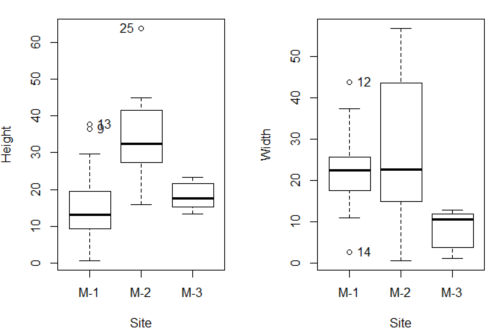
Figure 3. Box plots of growth responses of o`hia seedlings collected from three Maui sites, M-1 (elevation 750 ft), M-2 (elevation 1100 ft), and M-3 (elevation 6600 ft). Data adapted from Table 5 of Corn and Hiersey 1973.
R code to make Figure 4 plots
par(mfrow=c(1,2))
Boxplot(Height ~ Site, data = ohia, id = list(method = "y"))
Boxplot(Width ~ Site, data = ohia, id = list(method = "y"))
This dataset would typically be described as a one-way ANOVA problem. There was one treatment variable (population source) with three levels (M-1, M-2, M-3). From Rcmdr we select the one-way ANOVA: Statistics → Means → One-way ANOVA… and after selecting the Groups (from the Site variable) and the Response variable (e.g., Height), we have
AnovaModel.1 <- aov(Height ~ Site, data = ohia.ch12)
summary(AnovaModel.1)
           Df Sum Sq   Mean Sq  F value          Pr(>F)
Site        2   4070    2034.8    22.63 0.000000131 ***
Residuals  47   4227      89.9
---
Signif. codes: 0 '***' 0.001 '**' 0.01 '*' 0.05 '.' 0.1 ' ' 1
Let us proceed to test the null hypothesis (what was it???) using instead the lm() function. Four steps in all.
Step 1. Rcmdr: Statistics → Fit models → Linear model … (Fig 4)
Figure 4. R Commander, select to fit a Linear model.
Step 2. The pop up menu below (Fig. 6) follows.
First, What is our response (dependent) variable? What is our predictor (independent) variable? We then input our model. In this case, with only the one predictor variable, Sites, our model formula is simple to enter (Fig. 6): Height ~ Site
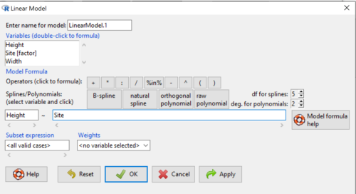
Figure 5. Input linear model formula
Step 3. Click OK to carry out the command.
Here is the R output and the statistical results from the application of the linear model.
LinearModel.1 <- lm(Height ~ Site, data=ohia.ch12)
summary(LinearModel.1)

Call:
lm(formula = Height ~ Site, data = ohia.ch12)

Residuals:
    Min     1Q   Median     3Q     Max
-18.808 -4.761   -1.755  4.758  29.257

Coefficients:
             Estimate  Std. Error  t value      Pr(>|t|)
(Intercept)    15.314       2.121    7.222 0.00000000377 ***
Site[T.M-2]    19.261       2.999    6.423 0.00000006153 ***
Site[T.M-3]     2.924       3.673    0.796          0.43
---
Signif. codes:  0 '***' 0.001 '**' 0.01 '*' 0.05 '.' 0.1 ' ' 1
Residual standard error: 9.483 on 47 degrees of freedom
Multiple R-squared:  0.4905,	Adjusted R-squared:  0.4688
F-statistic: 22.63 on 2 and 47 DF,  p-value: 0.0000001311
End R output
The linear model has produced a series of estimates of coefficients for the linear model, statistical tests of the significance of each component of the model, and the coefficient of determination, R2, which is a descriptive statistic of how well model fits the data. Instead of our single factor variable for Source Population like in ANOVA we have a series of what are called dummy variables or contrasts between the populations. Thus, there is a coefficient for the difference between M-1 and M-2. “Site[T.M-2]” in the output, between M-1 and M-3, and between M-2 and M-3.
Brief description of linear model output; these will be discussed fuller in Chapter 17 and Chapter 18. The residual standard error is a measure of how well a model fits the data. The Adjusted R-squared is calculated by dividing the residual mean square error by the total mean square error. The result is then subtracted from 1.
It also produced our first statistic that assesses how well the model fits the data called the coefficient of determination, R2. An of of 1.0 would indicate that all variation in the data set can be explained by the predictor variable(s) in the model with no residual error remaining. Our value of 49% indicates that nearly 50% of the variation in height of the seedlings grown under common environments are due to the source population (= genetics).
Step 4. But we are not quite there — we want the traditional ANOVA results (recall the ANOVA table).
To get the ANOVA Table we have to ask Rcmdr (and therefore R) to give us this. Select
Rcmdr: Models → Hypothesis tests → ANOVA table … (Fig 6)
Figure 6. To retrieve an ANOVA table, select Models, Hypothesis tests, then ANOVA table…
Here’s the type of tests for the ANOVA table, select the default (Fig 7)
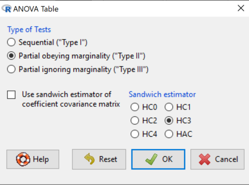
Figure 7. Options for types of tests.
Now, in the future when we work with more complicated experimental designs, we will also need to tell R how to conduct the test. For now, we will accept the default Type II type of test and ignore sandwich estimators. You should confirm that for a one-way ANOVA, Type I and Type II choices give you the same results.
The reason they do is because there is only one factor — when there are more than one factors, and if one or both of the factors are random effects, then Type I, II, and III will give you different answers. We will discuss this more as needed, but see the note below about default choices.
Marginal or partial effects are slopes (or first derivatives): they quantify the change in one variable given change in one or more independent variables. Type I tests are sequential: sums of squares are calculated in the order the predictor variables are entered into the model. Type II tests the sums of squares are calculated after adjusting for some of the variables in the model. Type III, every sum of square calculation is adjusted for all other variables in the model. Sandwich estimator refers to algorithms for calculating the structure of errors or residuals remaining after the predictor variables are fitted to the data. The assumption for ordinary least square estimation (See Chapter 17) is that errors across the predictors are equal, i.e., equal variances assumption. HC refers to “heteroscedasticity consistent” (Hayes and Chai 2007), which infers fitting of a model does not assume equal error variance across all observations.
By default, Rcmdr makes Type II. In most of the situations we will find ourselves this semester, this is the correct choice.
Below is the output from the ANOVA table request. Confirm that the information is identical to the output from the call to aov() function.
Anova(LinearModel.1, type = "II")
Anova Table (Type II tests)
Response: Height
          Sum Sq  Df   F value        Pr(>F)
Site      4069.7   2    22.626  0.0000001311 ***
Residuals 4226.9  47
---
Signif. codes: 0 '***' 0.001 '**' 0.01 '*' 0.05 '.' 0.1 ' ' 1
And the other stuff we got from the linear model command? Ignore for now but make note that this is a hint that regression and ANOVA are special cases of the same model, the linear model.
We do have some more work to do with ANOVA, but this is a good start.
Why use the linear model approach?
Chief among the reasons to use the lm() approach is to emphasize that a model approach is in use. One purpose of developing a model is to provide a formula to predict new values. Prediction from linear models is more fully developed in Chapter 17 and Chapter 18, but for now, we introduce the predict() function with our O`hia example.
myModel <- predict(LinearModel.1, interval = "confidence")
head(myModel, 3)    #print out first 3 rows
#Add the output to the data set
ohiaPred <- data.frame(ohia,myModel)
with(ohiaPred, tapply(fit, list(Site), mean, na.rm = TRUE))   #print out predicted values for the three sites
Output from R
myModel <- predict(LinearModel.1, interval = "confidence")
head(myModel, 3)
       fit      lwr      upr
1 15.31374 11.04775 19.57974
2 15.31374 11.04775 19.57974
3 15.31374 11.04775 19.57974
with(myModel, tapply(fit, list(Site), mean, na.rm = TRUE))
     M-1      M-2      M-3
15.31374 34.57474 18.23796
Questions
1. Revisit ANOVA problems in homework and questions from early parts of this chapter and apply lm() followed by Hypothesis testing (Rcmdr: Models → Hypothesis tests → ANOVA table) approach instead of one-way ANOVA command. Compare results using lm() to results from One-way ANOVA and other ANOVA problems.
Data set and R code used in this page
Corn and Hiesey (1973) Ohia common garden
| Site | Height | Width |
|---|---|---|
| M-1 | 12.5567 | 19.1264 |
| M-1 | 13.2019 | 13.1547 |
| M-1 | 8.0699 | 16.032 |
| M-1 | 6.0952 | 22.8586 |
| M-1 | 11.3879 | 11.0105 |
| M-1 | 12.2242 | 21.8102 |
| M-1 | 16.0147 | 11.0488 |
| M-1 | 19.7403 | 25.9756 |
| M-1 | 36.4824 | 25.2867 |
| M-1 | 13.1233 | 20.0487 |
| M-1 | 21.7725 | 24.8511 |
| M-1 | 14.2013 | 43.7679 |
| M-1 | 37.7629 | 37.3438 |
| M-1 | 2.8652 | 2.5549 |
| M-1 | 0.6456 | 22.8013 |
| M-1 | 29.623 | 20.0194 |
| M-1 | 10.5812 | 29.0328 |
| M-1 | 18.3046 | 22.2867 |
| M-1 | 19.0528 | 24.684 |
| M-1 | 2.5693 | 35.74 |
| M-2 | 45.0162 | 14.3878 |
| M-2 | 40.8404 | 18.8396 |
| M-2 | 27.1032 | 21.0547 |
| M-2 | 29.8036 | 16.9327 |
| M-2 | 63.8316 | 30.7037 |
| M-2 | 42.107 | 3.2491 |
| M-2 | 30.0322 | 47.4412 |
| M-2 | 34.0516 | 42.239 |
| M-2 | 15.7664 | 32.8354 |
| M-2 | 35.1262 | 50.9698 |
| M-2 | 43.6988 | 19.3897 |
| M-2 | 26.7585 | 13.8168 |
| M-2 | 36.7895 | 0.5817 |
| M-2 | 30.9458 | 53.7757 |
| M-2 | 26.8465 | 15.4137 |
| M-2 | 40.3883 | 9.2161 |
| M-2 | 30.6555 | 56.8456 |
| M-2 | 19.9736 | 44.9411 |
| M-2 | 27.676 | 36.8543 |
| M-2 | 44.084 | 24.3396 |
| M-3 | 15.2646 | 11.4999 |
| M-3 | 19.6745 | 9.7757 |
| M-3 | 23.275 | 12.7825 |
| M-3 | 16.1161 | 2.4065 |
| M-3 | 16.8393 | 1.1253 |
| M-3 | 23.107 | 3.7349 |
| M-3 | 21.5322 | 6.9725 |
| M-3 | 13.4191 | 12.2867 |
| M-3 | 14.7273 | 11.4841 |
| M-3 | 18.4245 | 11.9078 |