Install R Commander

Download pdf file of this page

Introduction

For beginning (bio)statistics students who need R, I recommend use of the graphic user interface, GUI, R Commander. R Commander is an R package. It’s a large package, and requires installation of many additional packages. Generally, these additional required packages are also installed with the installation of R Commander.

This page provides a guide about how to install R Commander onto your computer (LDE). To use R Commander, please see Chapter 1.1 – A quick look at R and R Commander. You must have R installed and working correctly on your computer before proceeding to install the R Commander package. Click here to get the Install R guide.

Installation guides quickly become outdated. This page last updated 12 August 2025 and describes working installation protocols at that time. Like all secondary guides to software installation, I recommend reading installation notes by the coders who provide the software. For R Commander, see R Commander Installation Notes, by Dr John Fox.

For your convenience, the example R code I run is listed below

myX <- c(1,2,3,4)
myY <- c(5,10,15,20)
plot(myY, myX)

For BI311, we also use R Commander

R Commander is a package that adds function to R; it provides a familiar point-and-click interface to R, which allows the user to access functions via a drop-down menu system (Fox 2017). Thus, instead of writing code to run a statistical test, Rcmdr provides a simple menu driven approach to help students select and apply the correct statistical test. R Commander also provides access to Rmarkdown and a menu approach to rendering reports.

RStudio is another way to interact with R, and compared to R Commander, is designed to help R programmers with a useful environment to manage files, generate reports, and work on R code. I continue to use R Commander in teaching because it emphasizes statistics and note coding. One advantage of R Commander for learning how to code with R is that code is reproduced from student’s selections in the drop-down menu options.

Install R Commander

To install R Commander, enter the following code at the R prompt. See Figure 1 below for a screenshot of the R Commander interface.

install.packages("Rcmdr")

In addition, download and install the plugin

install.packages("RcmdrMisc")

Note: You can combine requests as follows

install.packages("Rcmdr", "RcmdrMisc", dependencies=TRUE)

Adding “dependencies=TRUE” will also install other packages that Rcmdr needs (which would get downloaded once you start Rcmdr for the first time).

If you have not set a mirror site, you’ll be prompted to do so before you can download and install packages. I recommend 0-Cloud as default mirror site. Be advised: because our university shares a single public IP address, you may experience download delays if we all try to use the same mirror site at the same time.

To start R Commander, load the packages via the library() command.

library(Rcmdr)

Follow installation prompts. You can skip adding the “otools,” for now. However, Rcmdr will prompt you to install otools every time you start, so go ahead and install them at your convenience.

MacOS users: To improve Rcmdr performance you must turn off “app nap.” From Rcmdr, go to Tools, then select “Manage Mac OS X app nap for R.app …” Once you select “off” (click OK to apply), restart Rcmdr, the delay will be removed. Windows 11 folks don’t have to contend with nap.

Test Rcmdr

Figure 1 shows a basic R Commander session. Enter code in the script window (1), click on the Submit button to run the code, and results show up in the output window (2). Figure 1 shows R Commander opened in a MDI.

Figure 1. Screenshot of basic R Commander session on WinPC.

Click on R Markdown tab, edit (e.g., replace with your own title and name), then click on the Generate Report button to create a pdf of your work, default file name is RcmdrMarkdown.pdf (Fig 2). If you do not have pandoc and LaTeX properly installed, then only an HTML document will be available as an option.

Figure 2. Screenshot of portion of RcmdrMarkdown.pdf.

Although I don’t recommend this practice, you can run R Commander from within RStudio. The downside is that multiple windows may be generated (Fig 3), which can be challenging for new users to navigate. On Windows pc some of this behavior can be controlled by selecting the SDI windowing option as opposed to the default MDI windowing option.

Figure 3. Screenshot of basic R Commander session in RStudio on macOS.

Add pandoc and LaTex support

To complete your R Commander installation you may want to add additional document handling software, LaTex and pandoc. R Commander already contains R Markdown, but these additional software allow you to take advantage of “high-quality typesetting.”

In Rcmdr, select Tools from the menu, then Install Auxillary Software. Click OK, which will open links in your default browser to download pages for LaTex and pandoc. Download the files, follow the installation instructions for pandoc and LaTeX, then restart R and Rcmdr.

Here are direct links to the files, plus installation notes

LaTeX — links verified 27 August 2025

MikTeX from https://miktex.org/download:

• for Windows systems, select basic-miktex-24.1-x64.exe
• for MacOS, select miktex-22.1-darwin-x86_64.dmg

pandoc — links verified 12 August 2025

Windows 11

https://github.com/jgm/pandoc/releases/download/3.7.0.2/pandoc-3.7.0.2-windows-x86_64.msi

MacOS

ARM CPU (M1 – M4): https://github.com/jgm/pandoc/releases/download/3.7.0.2/pandoc-3.7.0.2-1-arm64.deb

INTEL CPU: https://github.com/jgm/pandoc/releases/download/3.7.0.2/pandoc-3.7.0.2-x86_64-macOS.pkg

/MD

14.7 – Rcmdr Multiway ANOVA

Introduction

We have been talking about the two-way randomized, balanced, replicated design.  Here, we take you step by step through use of R to conduct the multiway ANOVA.

R code: Multiway ANOVA

Rcmdr: Statistics → Means → Multiway ANOVA… we will review this as Option 1

or

Rcmdr: Statistics → Fit Models → Linear model… we will review this as Option 2

In either case, as a reminder, your data set must be stacked worksheet, like the data in this worksheet

Table 1. Data set, example.14.7†

Option 1

Your first option is to use the ANOVA menus via “Means.” This is a perfectly good way to handle a standard two-way, fully-crossed, fixed effects model.  However, other designs will not run with this command and R will return a report of errors for ANOVA models that do not conform to the replicated, balanced, crossed design.

Rcmdr: Statistics → Means → Multiway Analysis of variance …

Factors: highlight “Diet” AND “Population”

Response variable: pick one (in this window, all we see is “Response”)

Figure 1. Screenshot Rcmdr multi-way ANOVA.

Interpret the output

AnovaModel.2 <- (lm(Response ~ Diet*Population, data=example.14.7))

Anova(AnovaModel.2)
 
Anova Table (Type II tests)
Response: Response
                  Sum Sq    Df    F value      Pr(>F) 
Diet              36.750     1    12.2500    0.008079 **
Population        10.083     1     3.3611    0.104104 
Diet:Population   52.083     1    17.3611    0.003136 **
Residuals         24.000     8
---
Signif. codes: 0 '***' 0.001 '**' 0.01 '*' 0.05 '.' 0.1 ' ' 1 
tapply(example.14.7 Response, list(Diet=example.14.7 Diet, 
+ Population=example.14.7 Population), mean, na.rm=TRUE) # means
Population
Diet 1 2
A 5.00000 7.333333
B 12.66667 6.666667

tapply(example.14.7 Response, list(Diet=example.14.7 Diet, 
+ Population=example.14.7 Population), sd, na.rm=TRUE) # std. deviations
Population
Diet 1 2
A 1.000000 2.081666
B 2.081666 1.527525

tapply(example.14.7 Response, list(Diet=example.14.71 Diet, 
+ Population=example.14.7 Population), function(x) sum(!is.na(x))) # counts
Population
Diet 1 2
A 3 3
B 3 3

End R output.

Summary of multi-way ANOVA command

The multi-way ANOVA command returns our ANOVA table plus the adjusted means, along with standard deviations and number of observations (counts).  The adjusted means would then be good to put into a chart to present group comparisons following adjustments from the effects of levels within groups.

Rcmdr: Models → Graphs → Predictor effect plots …

Here’s the chart (hint: )

Figure 2. Predictor effect plots, Diet and Population on Response variable.

Option 2

A more general approach is to use the General linear model. This approach can handle the standard 2-way fixed effects ANOVA (above), but any other model as well. The model is Response ~ Diet*Population.

Rcmdr: Statistics → Fit Models → Linear model… 

Figure 3. Screenshot Rcmdr linear model menu.

Interpret the output

LinearModel.1 <- lm(Response ~ Diet * Population, data=example.14.7)

summary(LinearModel.1)

Call:
lm(formula = Response ~ Diet * Population, data = example.14.7)

Residuals:
Min 1Q Median 3Q Max 
-2.3333 -1.1667 0.1667 1.0833 2.3333 

Coefficients:
                        Estimate    Std. Error ..t value .  Pr(>|t|) 
(Intercept) .              5.000         1.000 .   5.000    .0.00105 ** 
Diet[T.B] .                7.667       ..1.414 .   5.421    .0.00063 ***
Population[T.2]           .2.333       ..1.414 .   1.650    .0.13757 
Diet[T.B]:Population[T.2] -8.333       ..2.000    -4.167    .0.00314 ** 
---
Signif. codes: 0 '***' 0.001 '**' 0.01 '*' 0.05 '.' 0.1 ' ' 1 

Residual standard error: 1.732 on 8 degrees of freedom
Multiple R-squared: 0.8047, Adjusted R-squared: 0.7315 
F-statistic: 10.99 on 3 and 8 DF, p-value: 0.003285 

End R output

Lots to sort through, so let’s begin with what is in common between the two approaches, the Multi-way ANOVA command versus the linear model command.

Compare R output from ANOVA and linear model

As a direct output, the linear model option does not provide an ANOVA summary table. Instead of our ANOVA table the linear model returns estimates of coefficients along with t-test results for each coefficient of the model from the lm() command output

Recall that we can get ANOVA tables through the following R commands via Rcmdr.

Rcmdr: Models → Hypothesis tests → ANOVA Table.

Let’s do so for this linear model (accept the default for type of tests = “Type II”).

And the output from lm() stored in the object LinearModel.1 is

Anova(LinearModel.1, type="II")
Anova Table (Type II tests)

Response: Response
                Sum Sq Df F value   Pr(>F)   
Diet            36.750  1 12.2500 0.008079 **
Population      10.083  1  3.3611 0.104104   
Diet:Population 52.083  1 17.3611 0.003136 **
Residuals       24.000  8                    
---
Signif. codes:  0 '***' 0.001 '**' 0.01 '*' 0.05 '.' 0.1 ' ' 1

End R output

Now, we’re in business, and, using the lm() function, we have the estimates for each model coefficient plus our ANOVA table.

Same answer! Of course. Which to choose, Option 1 or Option 2? Use the lm() options; more flexible, covers more designs than the multiway ANOVA which is strictly for the crossed fully replicated design.

Questions

1. Write out the two-way model described for the data in Table 1.
2. Write the null hypotheses and provide a summary of the statistical significance of the model.

Quiz Chapter 14.7

Rcmdr Multiway ANOVA

Start Quiz

Question

Confirm

✕

✓

Your answer:

Correct answer:

Next

Please wait..

↺

You got {{SCORE_CORRECT}} out of {{SCORE_TOTAL}}

Your Answers

Chapter 14 contents

• Introduction
• Crossed, balanced, fully replicated
• Sources of variation
• Fixed effects, Random effects
• Randomized block design
• Nested designs
• Some other ANOVA designs
• Rcmdr Multiway ANOVA
• More on the linear model in Rcmdr
• References and suggested readings

2.2 – Why do we use R Software?

If this page is TL;DR, and you’re in a rush, then instructions to install R onto your macOS or Windows PC are provided in Install R.  To run in the cloud only, see Use R in the cloud.

Why R? The case for using R in biostatistics education.

.

Why do we use R Software? Or put another way: DrD, Why are you making me use R?

Truth? You can use just about any acceptable statistical application to get the work done and achieve the learning objectives we have for beginning biostatistics. However, we will use the R statistical language as our primary statistical software in this course. Part of the justification is that all statistical software applications come with a learning curve, so you’d start at zero regardless of which application I used for the course.

In selecting software for statistics I have several criteria. The software should be:

• if not exactly easy, the software should have a reasonable learning curve
• widely accessible and compatible with all most personal computers
• well-respected and widely used by professionals
• free software
• open source
• well-supported for the purposes of data analysis and data processing
• really good for making graphics, from the basics to advanced
• capable to handle diverse kinds of statistical tests

R meets all of these criteria. R history began back in 1993 and has always been available as free software under the terms of the Free Software Foundation’s GNU General Public License in source code form. R compiles and runs on a wide variety of UNIX platforms and similar systems, including GNU/LINUX, FreeBSD, and various Linux distros like the popular Ubuntu^®, in addition to their more famous Microsoft Windows^® and Apple macOS^® distributions. To facilitate access to the software, numerous mirror sites are available from sites around the world, with cloud.r-project.org supported by RStudio perhaps the most widely used. From January 2024 to December 2024, more than 8.5 million downloads of base R were made from the RStudio CRAN mirror site (CRAN stands for Comprehensive R Archive Network.

install.packages("cranlogs")
library(cranlogs)
# How many downloads of base R around start of Fall semester?
 out <- cran_downloads("R", from = "2025-08-01", to = "2025-08-31")
sum(out$count)

[1] 582524

R is straightforward to use once you learn how to work with the language, but has a steep learning curve; after all, it’s a programming language. I recommend installing the program onto your computer, but ready to go R is also available at multiple cloud services, including Google CoLab and Posit Cloud. The remainder of this page is directed at users who choose to install R to their computer, although much of the discussion holds regardless of the R environment choice, local or Cloud.

For local installs of R, I also recommend use of the GUI R Commander.  Use of R Commander helps with the learning curve, and eventually, your use of code will become second nature. We don’t use RStudio, but as your skills improve, I recommend transitioning to the IDE RStudio; after the initial growing pains are behind you, RStudio likely will be a better solution over R Commander.

This discussion implies learning R programming. However, while we need statistical software to do statistics, students in my BI311 course must keep in mind that learning objectives for a biostatistics course is about the concepts and interpretation of statistics, not just use of the software. In other words, learning how to use R is not the focus of BI311 nor will you likely achieve R programming competency by the end of the semester. I certainly encourage students to strive for competency and I give frequent bonus opportunities to demonstrate coding skills during the semester.

Why R and not some other statistics software?

Thus, you might ask if the purpose of the course isn’t to learn R, why work with R instead of a more familiar app or software, eg, Microsoft Excel^® (hereafter simply referred to as Excel), or Google Sheets, or even my favorite open-source office alternative, LibreOffice Calc? Or, perhaps even just one of the many online calculators, if the course learning objective is to “just” learn about statistics?

First, I believe that real data derived from real biology or biomedical problems are essential elements to a first course in biostatistics. That’s not a particularly unique perspective although I don’t have survey results of other statistics instructors to back up the claim. Real problems involve observations on multiple subjects, many variables — large data sets; this alone precludes use of hand calculations and calculators. As a corollary, we will not spend a great deal of time learning the in’s and out’s of the algorithms that form particular statistical tests. Now, do understand that there is a tremendous benefit to understanding statistics by working through the equations, by looking at the algorithms, and there’s no escaping the need for understanding that probability provides the foundation of statistics inference (Chapter 8). Thus, for most of us, the statistical software available to us provides an appropriate framework for applying correct statistical tests to our projects. Therefore, the decision is about which statistical package we should use.

Second, R is perhaps the choice in academia for statistical software. A PUBMED search found more than 1500 citations of R. Visit Robert A. Muenchen’s web page (The popularity of data analysis software, r4stats.com) to see updated statistics on statistical software use. Those of you continuing on to graduate school or to professional schools will find that many of your statistically literate colleagues use R and not one of the commercial programs. While there are many excellent commercial packages (Table 1), and in some cases you can make spreadsheet programs do statistics (typically add-ins are required), all statistical software come with steep learning curves. Thus, part of my selling point to you is that learning to use R is at the cutting-edge in your field and, given that all of the software you could use can have have their challenges, it is best to work with something that will be around and is in wide use, without the burden of a financial investment.

Table 1. A selective list of statistical software.

see Wikipedia for list of additional software

Third, what about online sites like plot.ly where, for free, you can plot and, in some cases, calculate statistics? What about the web application at Brightstat, which claims to provide an SPSS-like experience online (Stricker 2008)? While it is true that there are many wonderful websites that can perform many of the statistical tests we will use this semester, these sites are not suitable for more than occasional use.

How to get started with R.

.

A few words about my approach to the software in my biostatistics course. I note to students during the semester that our course is not a programming course, but rather, programming skills are acquired along the way. Our focus is how to do statistical analysis, how to design experiments, etc. Coding skills without understanding of the why we’re doing it is not unlike learning to cook by following a great recipe as opposed to learning about the art and science of flavor (NPR Science Friday, March 15, 2024) — the homework is solved but the why we can support our conclusions may be obscure.

We set aside the first couple of class meetings simply to setup student’s Windows PC or Apple macOS computers to do data science; for students with access to Chromebooks or iPad tablets, we need to set them up to run R in the Cloud (eg., Google Colaboratory) — in other words, there’s a lot of pre-work that can present barriers to actual doing statistics in R (or other software). Once we have the environment set up for the students, we utilize a “tell-show-do” approach to learning how to code. The “tell” part includes sharing script; the “do” part is mostly done by students outside of class as part of completing homework.

First work with the language can be frustrating, so I also encourage a “five minute” rule — if it ain’t working, stop. So, by all means when Run through a troubleshooting checklist, but please don’t continue to struggle — the gap is between the instructions and where the student is with the material — it’s a me-as-instructor problem, not a student must work harder problem! 

All statistics work follows a similar workflow.

The basic workflow for a data project, using R as the primary statistical programming tool, looks like that illustrated in Figure 1.

Figure 1. A basic workflow with R.

The workflow begins with the assumption that a data set already exists. Getting the data into an R session depends on the source of the data, for example stored in spreadsheet file or from a table on a webpage. Data cleaning and processing of the data may be in order — for small and modest-sized data sets, my own preference is to do most of the data cleaning in my spreadsheet app, but R has full capabilities to handle or “wrangle” data. Next, the raw data should be stored in R session in a data frame object. Once the data frame object is available, exploratory data analysis, including summary statistics and data visualization can proceed. Higher order analytics, including statistical inference and modeling, can then begin.

The R statistical language, accompanied by additional packages to extend its capabilities beyond basic math and statistical functions, provided a complete statistical environment. R is best viewed as a programming language for statistics (data analysis), and data processing. Power users of R learn how to write scripts that do t-tests, ANOVA, regression, etc. The scripts are just lines of code that R understands and it provides the user tremendous control over analysis and inference of data sets. Because of this flexibility and power, however, R can be intimidating at first. So, we’ll start slowly with scripts, introducing just what we need to get started and build from there. We’ll be addressing R issues in more depth over the next several weeks, but for the first week, our goal(s) should be to make sure each of you knows how to start/exit R, how to create and utilize a working directory, and how to use R as a calculator. You obtain your copy of R from the R Project for Statistical Computing, available at https://www.r-project.org. Instructions to install R are provided in Install R.  A ten-part tutorial to get started using R is provided in Mike’s Workbook for Biostatistics.

 /Users/username/Desktop/BI311

Why R Commander, why not RStudio?

.

We utilize an R package that provides a menu-driven context to much of the typical statistics one needs to do biostatistics. The package is called R Commander (Rcmdr), which provides a graphic user interface or GUI. Rcmdr therefore significantly eases the learning curve for doing statistics with R. We use a package called R Commander, which provides drop down menus for most of the typical kinds of analyses. Rcmdr is in use in many courses across the world (more than 17K downloads in August 2025), and among the other GUI available for R, Rcmdr is among the best supported GUI available for R. R Commander function is extended by plug-ins; as of August 2025, there were 31 plugins that extend Rcmdr’s capabilities. Instructions to install R Commander are provided in Install R Commander. 

Wait! Why don’t we use Excel? My instructor in {insert course here} used Excel…

.

A very reasonable question for you to ask — why don’t we use Microsoft Excel or Google Sheets for statistics? Moreover, it is highly likely that you have gained at least some introduction to descriptive statistics and graphing with spreadsheets in former courses — shouldn’t we learn statistics within a software framework you are already familiar?

After all, “Can’t Microsoft Excel do statistics?” Mostly the answer is, no, not really (Fig 2).

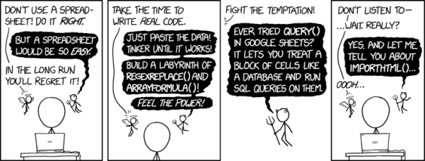
Figure 2. “Spreadsheets,” xkcd.com no. 2180.

MS Excel, Google Sheets, Apple Numbers, and for that matter, Calc, the spreadsheet application in my favorite office app LibreOffice (LibreOffice is a free, open-source alternative to Microsoft Office), can be used to calculate many descriptive statistics. With some effort, these applications can be extended by use of either Analysis ToolPak or Solver Add-ins to do more complicated statistics like regression and analysis of variance, and curve fitting.

However, use of MS Excel for statistical analysis involves learning a number of commands, syntax, and developing workflows that are neither intuitive nor standard. Some publishers have provided add-ins that are reportedly designed to simplify this process (eg, XLStat, UNISTAT, Real Statistics using Excel). None of these options are free and none are in use in any major way by scientists (see Robert Muenchen’s The popularity of data analysis software). The free add-ins of Analysis ToolPak and Solver may work for you if you own a Windows PC, but only Solver is included for the Mac versions of Excel. MacOS users may download and install StatPlus:MacLE, which is a limited, but free alternative to the Analysis ToolPak add-in; for a complete package a Pro version is available (licenses started at $89, web site: www.analystsoft.com/en/products/statplusmacle/).

An additional caution: you should be aware that there have been reports over the years that algorithms selected by Microsoft for Excel have not always been to industry standards (eg, McCullogh and Wilson 2005). In short, the fit of Excel and other spreadsheet apps for use in statistics is not a simple one. To do the kinds of statistics we will use routinely in class, Excel would need to be modified with add-ins, and the add-ins would be the result of programming by someone. And you would still need to learn how to write the code.

What about graphics? You may like Microsoft Excel’s ability to do graphics. Indeed, Excel, Google Sheets, and LibreOffice Calc can be used to generate many typical kinds of statistical plots. But again, in comparison to R, spreadsheet app graphics are limited and require a deal of effort to generate acceptable plots. I think you’ll be surprised at how straight-forward R is. Here’s an example, first rendered in Microsoft Excel, then in base R. And importantly, the kinds of plots Excel does well at are not necessarily the plots suitable for research publication. For example, Excel allows you to make bar charts easily, but cannot do box plots. Box plots are preferred over bar (column) charts for ratio scale data.

Statistics comparisons between R and MS Excel.

.

About that learning curve. Let’s compare R and MS Excel for basic functions common in data analysis. Similar conclusions hold for comparisons to Google Sheets and LibreOffice Calcs.

Table 2 lists the observations we can use to conduct comparisons of the applications.

A simple data set

One of the first steps in data analysis is to produce what are called descriptive statistics. Common descriptive statistics are the mean and the sample standard deviation. Let’s compare Excel and R for retrieving these two statistics.

With Excel, to calculate the arithmetic mean of 24 numbers, enter the values into a single column of 24 rows, then enter “=average(A2:A25)“, without the quotes, into a new cell of the spreadsheet. “A2:A25” refers to where data would be contained in column A rows 2 through 25. Typically the first row in a worksheet would contain the name of the variable, eg, “A.” Depending on the significant figures set, the estimate returned by Excel for the mean of A is 59.58333333.

Similarly, to obtain the standard deviation, type =stdev(A2:A25), into a new cell of the spreadsheet. Again, depending on the significant figures set, Excel returns a value of 37.05215674 for the standard deviation of A.

In contrast, to obtain the mean and standard deviation for a variable in an R data set, all you would type at the R prompt (>), or in the script window

and then submit the code is:

myA <- c(12, 14, 20, 25, 28, 29, 32, 34, 35, 39, 47, 47, 50, 53, 54, 71, 79, 87, 89, 96, 105, 122, 130, 132)

where the “c” is a function to combine arguments into a vector and saved to the object myA, followed at the new line by

mean(myA)

Hit enter after entering the command) and R returns

[1] 59.58333

For the standard deviation, write the R base function sd()

sd(myA)

Hit enter after entering the command and R returns

[1] 37.05216

It’s not much of a difference, but note that to get the mean (arithmetic average) I typed seven characters in R, but 16 characters in Excel; similarly, for the standard deviation I typed in 5 characters in R, but 13 characters in Excel. That’s a savings of 56% and 62%, respectively. Excel tries to help by using AutoComplete to anticipate what you want to enter, but AutoComplete doesn’t always work properly (eg, see gene name errors generated by use of default Microsoft Excel settings, Ziemann et al 2016).

In conclusion, R is quicker for descriptive statistics.

Graphics comparison between R and MS Excel.

.

MS Excel is often cited for its graphics capabilities (Camões 2016). We can make the familiar scatter plots, bar charts, and pie charts in Excel. These plots and more are easily obtained in R. I won’t elaborate here about graphics, we talk at some length about graphics in Chapter 4. But here’s one example in R.

Let’s plot myB vs myA. We already provided the data for variable A, here’s the data for variable B.

17, 21, 21, 26, 27, 32, 28, 42, 40, 30, 71, 53, 56, 61, 55, 89, 82, 63, 116, 162, 116, 154, 137, 149

Don’t recall how to assign a set of numbers to an object, B, in R? See above and look again at how we assigned the numbers to object myA.

To get a simple scatter plot (Fig 3), I may write at the R prompt.

plot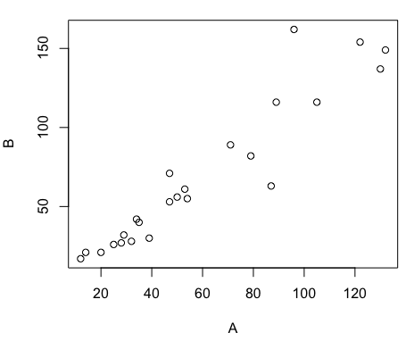(myA,myB)

Figure 3. Basic scatter plot made in R, plot(myA,myB).

And here’s the comparable default plot (Fig 4) from Microsoft Excel, Office 365

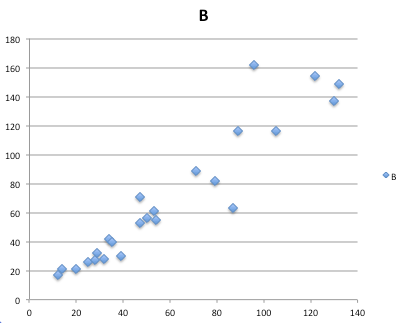
Figure 4. Basic scatterplot made in Microsoft Excel.

Now, both graphs need some work, and to be fair, these are just the defaults. With some effort, you can make an Excel graph look pretty good. But note — the defaults in Excel don’t generate axis labels, while R default plot does. Excel adds a useless title and legend; both need to be removed. Excel also adds grid lines where typically one would not include these in a scientific plot; for example, in the case of scatterplots, grid lines can distract the viewer from the data points and reduce the data-to-ink ratio Tufte 1984).

Count the steps to generate an acceptable scatter plot (Table 3). I’ve also added R Commander (Rcmdr) steps for comparisons (Rcmdr lets you use drop-down menus like Excel or Google Sheets or LibreOffice Calcs).

Table 3. Steps needed to make a simple scatterplot in R, R Commander, or Microsoft Excel.

Conclusion? R is quicker for routine statistical plots like a scatter plot. And I didn’t even count the steps needed to change MS Excel’s dreadful diamond icon points.

That’s one step in R, four steps in Rcmdr, but eight steps for Microsoft Excel. LibreOffice Calc is a little better at only four steps, but like MS Excel, you’d need to change several components to the graph (Fig 5).

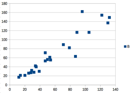
Figure 5. Basic scatterplot made in LibreOffice Calc.

plot(myA,myB, pch = 22)

So, you’re telling me I don’t need a spreadsheet application?

.

No, not at all. We use spreadsheets, and more generally, databases, to store data. Spreadsheets apps are designed to make data entry and data management approachable and efficient. They remain an important tool for researchers (Browman and Woo 2017).

R is not that great of a spreadsheet; packages are available to seamlessly tie your spreadsheet and database data to R via ODBC. We will routinely enter and manipulate data in MS Excel, then import the data into R for analysis.

Spreadsheet apps like MS Excel and Google Sheets (see also LibreOffice Calc) are great at being a spreadsheet program, R is great at being a statistical software program. You should take advantage of what the tools do best.

Still not convinced?

.

R is in use all over the world, by students and professionals alike and if one is going to spend the time to learn how to use a statistics software program, you should learn a standard program, like R.

And it’s not just me. Read about R in this 2009 New York Times piece, “Data analysts captivated by R’s power.” Look who purchased (April 2015) Revolution Analytics, a major player in the development of the R programming language.

Why install R on your computer?

.

Convenience. Control. Offline.

At the Biology department of Chaminade University, we have installed and maintain R, Rcmdr, and RStudio along with all required packages on our Macbook Pro® Lab computers for your use during class and during optional, proctored biostatistics work sessions. Since 2018, R is increasingly available “in the cloud” (eg, RStudio Cloud), which would mean you could run R in your browser and avoid installation on your computer. You can run significant analysis with R in the cloud via the free Google Colaboratory and CoCalc are now available: I encourage you to look into these platforms. Unfortunately, these services are not quite ready for the classroom. For example, RStudio in the Cloud is free to use on a limited basis, but quickly requires a significant subscription cost with increasing use. Google Colab and GoCalcs require use of Jupyter notebooks, which add yet another layer to the learning curve without focusing on learning statistics. Second, although access to their servers is easy, running simultaneous connections via Chaminade’s single public IP address is likely to lead to problems for us. Third, I want you to use R Commander (Rcmdr) to assist in the learning curve — Rcmdr cannot be run in the Cloud (ie, RStudio in the Cloud, Google Colaboratory, or CoCalc).

Therefore, you are encouraged to install R, Rcmdr, and even RStudio, onto your own computers, in part because of the convenience, but also because R is not generally available to students on campus, ie, only the Biology department’s computers have the up-to-date R software installed.

To get started, go to your Canvas website and view How to install R on your own computer.

An additional benefit to installing a version of R on your computer, you’ll understand more about the software if you take the time to install and if need be, troubleshoot your installation of the software. Moreover, there’s a considerable amount of help out there for R. For example, a simple Google search(keywords: tutorial “install R”), returns more than 700K hits, and more than 40K January 2023 alone (add “after:2023-01-01” to Google search box). In fact, there’s so much out there that you’ll want to sample from several sites and select the voice that works best for you.  

Questions

1. Write up three learning outcomes for this page. Hint: Point your favorite generative AI to this page and ask for help.
2. I listed several spreadsheet apps: Microsoft Excel, Google Sheets, Apple Numbers, LibreOffice Calc. Which of these are free to download and install to your computer? Which are freely available via the Cloud?
3. What level of confidence do you have to this statement: I am confident in my ability to use spreadsheet apps for my BI-311 work this semester. Response options: 
   1. Strongly disagree.
   2. Disagree.
   3. Agree.
   4. Strongly agree.
4. What level of confidence do you have to this statement: I am confident in my ability to use the R programming software for my BI-311 work this semester. Response options: 
   1. Strongly disagree.
   2. Disagree.
   3. Agree.
   4. Strongly agree.

.

Quiz Chapter 2.2

Why do we use R software?

Start Quiz

Question

✕

✓

Your answer:

Correct answer:

Next

Please wait..

↺

You got {{SCORE_CORRECT}} out of {{SCORE_TOTAL}}

Your Answers

Chapter 2 contents

.

• Introduction
• Why biostatistics?
• Why do we use R Software?
• A brief history of (bio)statistics
• Experimental Design and rise of statistics in medical research
• Scientific method and where statistics fits
• Statistical reasoning
• Chapter 2 – References and suggested reading

1.1 – A quick look at R and R Commander

A first look at R.

R is a programming language for statistical computing (Venables et al 2009). R is an interpreted language — when you run (execute) an R program — the R interpreter intercepts and runs the code immediately through its command-line interface, one line at time. Python is another popular interpreted language common in data science. Interpreted languages are in contrast to compiled languages, like C++ and Rust, where program code is sent to a compiler to a machine language application. R is free to use and available via many platforms, from local installations on a person’s laptop to running on cloud servers (Fig 1).

Figure 1. Choose how you will interact with R: on your computer (Blue box) or in the cloud (Red box). Users of Linux, macOS, and WinPC can either install R to their computer or choose to access R in the cloud (and/or, black arrow).

Before you begin, you have a choice: how do you want to work with R (Fig 1)? In part, the choice depends on your computing device. If you have a desktop or laptop computer, running Linux, Apple macOS, or Microsoft Windows, then R can be installed onto your computer (blue box, Fig 1). If, however, you have a ChromeBook, Apple iPad or iPhone, or any Android Tablet or Smartphone, you would go with the second option (red box, Fig 1).

For those going with installing R to their computer, the second choice is to pick the environment for creating and running scripts and managing file input and output during a session. Working environments for R in the cloud include RStudio and Jupyter Notebooks (eg, Google CoLab) (red box, Fig 1 — see Note 2 below). For installed R, two suggested environments are R Commander and RStudio, an Integrated Development Environment or IDE, RStudio (Fig 1). The choice depends on your needs — an IDE is helpful when you plan to write a lot of code, it’s a comprehensive programming environment, which includes many tools that support writing code from scratch.

For our course at Chaminade University, I recommend R Commander because of the drop-down menu approach to accessing statistical functions in R; R Commander is not a comprehensive environment, but it provides the necessary scripting window along with access to markdown editing. R Commander, Rcmdr, is an R package that provide a graphical user interface or GUI for R. It is based on the tcltk package. R must be installed first before installing the R Commander package. R Commander provides familiar menu functions, like many commercial statistical software. R Commander, like the IDE RStudio, is not necessary for R programming or conducting statistical analysis or even generating reports via markdown. R Commander, however, shrinks the learning curve with R programming basics so that students can focus on learning statistics, which is the chief objective of the Biostatistics course at Chaminade.

The following steps user through use of R and R Commander, from installation to writing and running commands. Mike’s Workbook for Biostatistics has a ten-part tutorial, A quick look at R and R Commander, which I recommend.

Install R.

.

Full installation instructions are available at Install R, and for the R Commander package, at Install R Commander. Here, we provide a brief overview of the installation process.

Download a copy of the R installation file appropriate for your computer from one of the Comprehensive R Archive Network (CRAN) mirror site of the r-project.org. For Hawaii, the most convenient mirror site is provided by the folks at RStudio (https://cloud.r-project.org/. In brief, Windows 11 users download and install the base distribution. MacOS users must first download and install XQuartz (https://Xquartz.org), which provides the X Window System needed by R’s GUI (graphic user interface). Once XQuartz is installed, proceed to install R to your computer. MacOS users — don’t forget to drag the R.app to your Applications folder!

Start R.

.

The following is a minimal look at how to use R and R Commander. Please refer to tutorials at  Mike’s Workbook for Biostatistics (R work, part 1 – 10) to learn use of R and R Commander.  

We’re just getting started, so the next thing to learn is how to set your working environment for your R sessions. Although we’ll discuss the R environment more as we proceed, it’s a good idea to start with a best practice action common in data science — always create and work from a working folder. This can be a local folder on your computer or pointed to a folder in your cloud storage. On my mac I usually create a folder on the desktop, example BI-311, and point to that as my working folder for a project. Now, we need to point R to use the working folder — we do this at start of each R session (or modify some code R needs during start up to always point to the folder — for now, we leave that for a later exercise). 

Once R is installed on your computer, start R as you would any program on your computer. For example, the icon for the R.app as it appears in the dock on a MacBook is shown in Figure 2.

Figure 2. R.app icon shown on a MacBook dock.

To point R to our working folder, there are several options. For now, we’ll go with writing and submitting a simple function in R. Recall that R has a command-line. The R prompt appears on the command line in the RGUI as the greater-than typographical symbol “>” at the beginning of a line (Fig 2). The prompt is returned by R to indicate the interpreter is ready to accept the next line of code.

First, discover where R is pointing to by submitting (type the command exactly as written then select keyboard shortcuts on Windows enter, or on macOS return key) the function getwd() at the prompt.

Ready to

On my MacBook, R returns

> getwd()
[1] "/Users/[username]/Documents"

To point to my working folder, I submit setwd("/Users/[username]/Desktop/BI311". When I run getwd() again, R returns the update

> getwd()
[1] "/Users/[username]/Desktop/BI311"

Ready to do some work?

R coding practices in this book and in the companion workbook roughly follow guidance outlined in a September 2018 R-Bloggers post, “R Code — Best practices,” by The R Trader. Of note, naming conventions: variables are nouns, variable names are written in lowerCamelCase; functions are verbs, function names are period separated, eg, my.function; script file names all end with .R and are written snake_case.R. Comments, preceded by #  and a single space, eg, # A brief comment, are sparingly included in code, but reserved for explanatory sentences in the text. We use <- and not = for assignment statements.

Where discussion requires reference to instructions on use of the R programming language, R code (instructions) the user needs to enter at the R prompt are shown in code blocks.

Courier New font within a “code block.”

Until you write your own functions, the general idea is, you enter one set of commands at a time, one line at a time. For example, to create a new variable, curryPoints, containing points scored by the NBA’s Steph Curry during the 2016 playoffs, type the following code at the R prompt (displayed as >, the “greater than” sign)

curryPoints <- c(24,6,40,29,26,28,24,19,31,31,11,18,19)

.

and to obtain the mean, or arithmetic average, for curryPoints at the R prompt type and enter

.

mean(curryPoints)

.

Output from R function mean will look like the following

.

[1] 24.42857

.

Functions in R, or any other data science programming language, are intended to automate a task.

df.curryPoints <- data.frame(curryPoints)

The R prompt appears in the RGUI as the greater-than typographical symbol “>” at the beginning of a line (Fig 3). The prompt is returned by R to indicate the interpreter is ready to accept the next line of code.

Figure 3. The R GUI on a macOS system; red arrow points to the R prompt.

Everything that exists is an object.

.

A brief programmer’s note — John M. Chambers, creator of the S programming language and a member of the R-project team, once wrote that sub-header phrase about R and objects. What that means for us: programming objects can be a combination of variables, functions, and data structures. During an R session the user creates and uses objects. The ls() function is a useful R command to list objects in memory. If you have been following along with your own installed R app, then how many objects are currently available in your session of R? Answer by submitting ls(). Hint: the answer should be one object.

A routine task during analysis is to calculate an estimate then use the result in subsequent work. For example, instead of simply printing the result of mean(curryPoints), we can assign the result to an object. 

myResult <- mean(curryPoints)

.

To confirm the new object was created, try ls() again. And, of course, there’s no particular reason to use the object name, myResult, I provided! Like any programming language, creating good object names will make your code easier to understand.

When you submit the above code, R returns the prompt, and the result of the function call is not displayed. View the result by submitting the object’s name at the R prompt, in this case, myResult. Alternatively, a simple trick is to string commands on the same line by adding ; (semicolon) at the end of the first command. For example,

myResult <- mean(curryRoints); myResult

.

Objects created during an R session, like curryPoints, are stored in memory within the Global Environment. To remove an object, use the command rm(myVariable). Why remove objects during an R session? If you are attempting multiple tasks in a homework assignment, removing unneeded objects helps maintain a clean and organized workspace, improving code readability and reducing the chance of accidental errors. 

Write your code as script.

.

While it is possible to submit code one line at a time, a much better approach is to create and manage code in a script file. A script file is just a text file with one command per line, but potentially containing many lines of code. Script files help automate R sessions. Once the code is ready, the user submits code to R from the script file.

Figure 4 shows how to create a new script file via the RGUI menu: File → New script.

Figure 4. Screenshot of drop down menu RGUI, create new script, Windows 11.

The default text editor opens (Fig 5).

Figure 5. Screenshot of portion of R Script editor, Windows 11. A simple R command is visible.

Submit code by placing cursor at start of the code or, if code consists of multiple lines, select all of the code, then hit keyboard keys Ctrl + R (Windows 11) or for macOS, Cmd + Enter.

I recommend starting with a clean environment, by using rm(list = ls()) at the beginning of a script.

By default, save R script files for reuse with the file extension .R, eg, my_script.R. Because the scripts are just text files you can use other editors that may make coding more enjoyable (see RStudio in particular, but there are many alternatives, some free to use. A good alternative is ESS).

Install R Commander package.

.

By now, you have installed the base package of the R statistical programming language (see for detailed instructions). The base package contains all of the components you would need to create and run data analysis and statistics on sets of data. However, you would quickly run into the need to develop functions, to write your own programs to facilitate your work. One of the great things about R is that a large community of programmers have written and contributed their own code; chances are high that someone has already written a function you would need. These functions are submitted in the form of packages. Throughout the semester we will install several R packages to extend R capabilities. R packages discussed in this book are listed at R packages of the Appendix.

Our first package to install is R Commander, Rcmdr for short. R Commander is a package that adds function to R; it provides a familiar point-and-click interface to R, which allows the user to access functions via a drop-down menu system (Fox 2017). Thus, instead of writing code to run a statistical test, Rcmdr provides a simple menu driven approach to help students select and apply the correct statistical test. R Commander also provides access to Rmarkdown and a menu approach to rendering reports.

install.packages("Rcmdr")

.

In addition, download and install the plugin 

install.packages("RcmdrMisc")

See Install R Commander for detailed installation instructions.

Start R Commander.

.

After installing Rcmdr, to start R Commander, type library(Rcmdr) at the R prompt and enter to load the library

library(Rcmdr)

.

On first run of R Commander you may see instructions for installing additional packages needed by R Commander. Accept the defaults and proceed to complete the installation of R Commander. Next time you start R commander the start up will be much faster since the additional packages needed by R Commander will already be present on your computer.

Note that you don’t type the R prompt and, indeed, in R Commander Script window you won’t see the prompt (Fig 6). Instead, you enter code in the R Script window, then click “Submit” button (or Win11: Ctrl+R or for macOS: Cmd+Enter), to send the command to the R interpreter. Results are sent to Output window (Fig 6). 

Figure 6. The windows of R Commander, macOS. From bottom to top: Messages, Output, Script (tab, Markdown) Rcmdr ver. 2.4-4.

Figure 6 shows how the R Commander GUI looks on a macOS computer. The look is similar on Microsoft Windows 11 machines (Fig 7).

Figure 7. The windows of R Commander, Win11. From bottom to top: Messages, Output, Script (tab, R Markdown) Rcmdr ver. 2.5-1.

We use R Commander because it gives us access to code from drop-down menus, which at least initially, helps learn R (Fox 2005, Fox 2016). Later, you’ll want to write the code yourself, and RStudio provides a nice environment to accomplish your data analysis.

Improve Rcmdr experience.

Windows users: R Commander works best in Windows if SDI option is set. This can be accomplished during R installation (“Startup options” popup, change from default “No” to “Yes” to customize), but you can also change after installing R. Win11 users should change from MDI to SDI — from one big window to separate windows — (see Do explore settings, WinPC see Fig 9; macOS see Fig 10). The downside of SDI is that while multiple Windows may appear during an R session, one or more windows may be hidden by an open window. For example, plots will popup in a new window and may be obscured by the Rcmdr window if full screen. A simple trick to view active windows on Win11 is to use the keyboard shortcut s Alt + Tab to view and cycle between windows. What about SDI and RStudio? RStudio experience will be similar whether MDI (default) or SDI was selected.

macOS users: To improve R Commander performance, turn off Apple’s app nap (see Do explore settings, Figures 6), which should improve a Mac user’s experience with R Commander and other X Window applications.

Complete R setup by installing LaTeX and pandoc for Markdown.

.

LaTeX is a system for document preparation. pandoc is a document converter system. Markdown is a language used to create formatted writing from simple text code.  Once these supporting apps are installed, sophisticated reports can be generated from R sessions, by-passing copy and paste methods one might employ. See Install R Commander for instructions to add these apps.

R Markdown.

.

Markdown is a syntax for plain text formatting and is really helpful for generating clean html (web) files.  R Commander also helps us with our reporting. R Markdown is provided as a tab (Fig 6, Fig 7). Provided you have also installed pandoc on your computer, you can also convert or “render” the work into other formats including pdf and epub. Unsure if your computer has pandoc installed? If you are unsure than most likely it is not installed. 😁 Rcmdr provides a quick check — go to Tools and if you see Install auxiliary software, then click on it and a link to pandoc website to find and download installation file.  You can also confirm install of pandoc by opening a terminal on your computer (eg, search “terminal” on macOS or “cmd” on Win11), then enter pandoc –version at the shell prompt. Figure 8 shows version pandoc is installed on my Win11 HP laptop.

Figure 8.  Screenshot of terminal window (cmd) on win11 computer, checking for installed pandoc on a win10 pc.

Enter your R code in the script window, submit your code, and your results (code, output, graphs) are neatly formatted for you by Markdown. Once the Markdown file is created in R Commander, you can then export to an html file for a a web browser, an MS Word document, or other modes.

Do explore settings!

.

After installation, R and R Commander are ready to go. However, students are advised that a few settings may need to be changed to improve performance. For example, on Win11 PCs, R Commander recommends changing from the default MDI (Multiple Document Interface) to SDI (Single Document Interface).  Check the SDI button via Edit menu, select GUI preferences menu.  Click save, which will make changes to .RProfile, then exit and restart R. Check to make sure the changes have been made (Fig 9). 

Figure 9. Screenshot of GUI preferences settings after changing from default MDI to SDI, win10

For macOS users, both R and Rcmdr will run better if you turn off Apple’s power saving feature called nap. From Rcmdr go to Tools and select Manage Mac OS X app nap for R.app… (Fig 10).

Figure 10. Screenshot Rcmdr Tools popup menu, macOS 10.15.6

A dialog box appears; select off to turn off app nap (Fig 11).

Figure 11. Screenshot Rcmdr Set app nap dialog box, macOS 10.15.6

Exit R Commander.

.

Click on Rcmdr: File → Exit, then choose to exit from just R Commander, or both R Commander and R.

If you exit just R Commander or both R and R Commander, you’ll receive a pop-up request to confirm you want to quit R Commander (click yes), and a second prompt asking if you want to save your script. In general, select yes and then you’ll be able to take up where you left off. Similarly, if asked to save your workspace, choose no. If you save workspace, this creates an .RProfile text file with settings for how R and R Commander will behave the next time you start R. The file will be saved to your current working folder, which R will use the next time R starts. At least while you are getting started, you should avoid creating these .RProfile files.

As long as the current session of R is active, then the library for Rcmdr, as well as any other library loaded during the R session, is in memory. To start R Commander again while R is running,  at the R prompt, type and submit

Commander()

Questions.

1. Biostatistics students should work through my ten R lessons, A quick look t R and R Commander, available in Mike’s Workbook for Biostatistics.
2. Students should also search Internet for R tutorials and R Commander tutorials. Find recent tutorials and work through several of them. We get better when we practice.

Quiz Chapter 1.1

A quick look at R and R Commander

Start Quiz

Question

✕

✓

Your answer:

Correct answer:

Next

Please wait..

↺

You got {{SCORE_CORRECT}} out of {{SCORE_TOTAL}}

Your Answers

Chapter 1 contents

.

• Getting started
• A quick look at R and R Commander
• Chapter 1 – References

Preface

Overview.

.

The following pages, loosely called Mike’s Biostatistics Book, contain the extended versions of my lectures for BI311 Biostatistics, a biology course I teach at Chaminade University. 

The companion site, Mike’s Workbook for Biostatistics, provides homework, problems and projects to learn-by-doing biostatistics, and several R tutorials. (I’ve also put together a number of handouts, background, and bioinformatics support at Mike’s Genetics & Genomics Workbook, consisting of materials used to support my lab classes these past 20 years.)

The Biology department faculty require biology majors to take this course. Class standing of students range from sophomores to first year graduate students.

We use and rely heavily on R, the open source “language and environment for statistical computing” (R-project [dot] org), and the R Commander package by J Fox (Fox 2005; Fox 2016). R Commander allows students to gain confidence with R commands by use of drop down menus to access functions. Increasingly, we also use Google CoLab to run simple R sessions.

The lecture notes are written from my perspective on what matters in a semester-long, first course in Biostatistics: concepts, context and practical advice along with a generous introduction to general linear models. The focus is on applied statistics with reference to other data science skill sets as needed. Concepts are illustrated by examples and multiple choice questions to “test” reader comprehension. Examples in Mike’s Biostatistics Book are generally from real data sets in biological or biomedical research. Therefore, context and practice comes from data sets we will work on throughout the semester.  The data sets are presented in the accompanying workbook, body titled Mike’s Workbook for Biostatistics.

The material presented in Mike’s Biostatistics Book provide background and the examples needed to complete the problems presented in the course workbook.

• Chapter 2: Statistical reasoning.
  • Workbook: Homework 1: Project data life cycle.
• Chapter 3 and 4: Exploring data.
  • Workbook: Homework 2A: Descriptive statistics.
  • Workbook: Homework 2B: Graphs.
• Chapter 5: Experimental design.
• Chapter 6: Probability.
  • Workbook: Homework 3: Distributions & Probability.
• Chapter 7: Risk analysis.
  • Workbook: Homework 4: Risk.
• Chapter 8: Inferential statistics.
  • Workbook: Homework 5: Inference.
• Chapter 9: Qualitative (categorical) analyses.
  • Workbook: Homework 6: Chi-square problems.
• Chapter 10 – 19: Quantitative (continuous) analyses.
  
  • Chapter 10, 12, 13 – Workbook: Homework 7: t-tests and ANOVA.
  • Workbook: Homework 8: Multiway ANOVA.
  • Workbook: Homework 10: Correlation.
  • Workbook: Homework 10: Multiple linear regression.
  • Chapter 11: Power analysis.
  • Chapter 15: Nonparametric tests.
  • Chapter 19: Distribution-free methods.
• Chapter 20: Additional topics (partial listing).
  • growth curves, dose response.
  • logistic regression.
  • others.
• Statistical tables.
• Appendix
  • Install R

While the intention is to downplay lists of statistical tests in favor of developing statistical reasoning, many of the kinds of tests one comes across are introduced and discussed in this book. The intent is to introduce these tests as special cases of general (or generalized) models from a data analyst’s point of view. Think of “k-means clustering“, “independent sample t-test“, “ANOVA“, “linear regression“, and the other tests as vocabulary. We understand biology best when we can talk the talk, and the same holds for learning statistics.

The book does not include machine learning — systems that can learn and help make decisions from data — and as of September 2023, includes only a short discourse on clustering and dimensionality reduction of data sets.

About this book (and website).

.

This textbook is an eBook and will undergo updates to correct errors, improve clarity, and even new content, throughout the semester. Although in spirit I welcome comments, corrections, and suggestions to improve coverage and content, I have closed comments at this site to minimize spam. As the book has a modest readership from multiple countries, I’m always happy to try and answer student questions — A little judicious search on the part of the reader likely will find a relevant email address.

Typesetting.

.

The manuscript was type set from a mix of html and Markup language — See Part 09: Making a report at Mike’s Biostatistics Book — and Ghostwriter (version 2 [dot] 1 [dot] 1), and the eBook (pdf version coming soon!) was generated and edited with Calibre (version 5 [dot] 35 [dot] 0).

Text to speech considerations.

Text to speech apps can get confused when a period appears within text and not just at the end of a sentence. Therefore, I’ve dropped periods from “Fig. 1” and the “e.g.” and “i.e.” Latin abbreviations. Periods appear in R commands, for example, data.frame(), and those remain as is. Similarly, I generally add a period after a subheading to encourage a break by text to speech apps.

Hosting.

Both books, Mike’s Biostatistics Book and Mike’s Workbook for Biostatistics, are hosted on my website. This site, Mike’s Biostatistics Book, is solely supported by me and I don’t monetize the site. As of  Fall 2023, the site cookie only stores temporary session information during a users visit.

Equations.

.

Equations in the eBook were created with LaTeX — a software system used to prepare and format documents — and saved as PNG images, or embedded in text (QuickLaTeX WordPress plug-in). Pages with many images or equations may be slow to load in your browser: in general, to improve browsing experience reduce the number of open tabs and use of additional apps.

References and citations.

.

Introductory textbooks often lack in-line citations. The absence of in-line citations improves readability, but at the very real expense of giving credit to the original and to providing the reader the opportunity to verify facts and opinions presented. I have tried a balance: first, I included in-line citations to references. One of many remaining tasks for me to improve the book is to complete linkage of in-page citations to reference lists. I have, however, refrained from an exhaustive, dissertation-like reference listing for each point raised in the book. Second, most citations are to open access articles (or articles with pdfs available by judicious search), with the justification of the reader has access to the original material. However, this approach is a form of citation bias.  Thus, I refer to reference pages as References and Suggested Readings, and don’t claim Mike’s Biostatistics Book as an authoritative voice on the subject (cf. discussion in Greenberg 2009 Bmj 339). 

A note about me.

.

I’m an Associate Professor of Biology at Chaminade University. My PhD was not in statistics, I trained in evolutionary physiology and quantitative genetics. Quantitative genetics is an applied field that depends heavily on use of mathematics and statistics, particularly linear models. I took courses in applied statistics while at the University of Wisconsin, but I would not call my training in statistics thorough or complete. Much of what I know comes from self-study. My strengths in biostatistics, I believe, are in translation of sometimes dense mathematics to direct use and application. Thus, I have developed a direct style to the material that I hope you will find helpful as you work on the material. It also means we won’t spend a lot of time with proofs, not because these are unimportant, but because they can side-track from developing your statistical thinking when it comes to data analysis — but primarily because this is not my strength. References are presented in the book to support the algorithms and mathematical foundations of biostatistics and to back claims I make about applied statistics.

Thus, I don’t claim that I have all of the answers, nor am I saying that the mathematical foundations are unimportant, far from it. But we have to start somewhere and I elect to spend our time on the concepts in statistics, the why do we do it this way, as opposed to the mechanics of the mathematics, the how do we do it.

What I have learned about statistics comes from publications from many real statisticians; Mike’s Biostatistics Book, such as it is, stands on on their work. I apologize in advance to any author whose work has not been given proper credit. Mistakes or mischaracterizations are, of course, mine alone.

Other sources of expertise.

.

Mike’s Biostatistics Book of lecture notes is intended to provide students with a foundation in biostatistics: the concepts of assumptions, probability, sampling, description, and modeling that support a researcher’s ability to advance knowledge in biology. But you will very much benefit from other opinions, other voices. And, as much as I have adopted the online presence, it is hard to beat a book in hand as a guide. Good statistics books retain their value well passed their publication date. Some of the textbooks I have found useful over the years include the following:

Introduction and general statistics.

.

Chaterjee S, Price B (1977) Regression analysis by example. Wiley Interscience (5th edition now published in 2006)

Glover T, Mitchell K (2008) Introduction to biostatistics, 2nd edition. Waveland Press

Norman GR, Streiner DL (2003) PDQ Statistics, 3rd edition. BC Decker

Snedecor GW, Cochran WG (1989) Statistical methods, 8th edition. Iowa State University Press

Sokal RR, Rohlf (1981) Biometry, 2nd edition. WH Freeman (4th edition published in 2011)

Whitlock MC, Schluter D (2008) The analysis of biological data. Roberts and Company

Zar J (1999) Biostatistical analysis, 4th edition. Prentice Hall (5th edition published in 2011)

Intermediate and advanced books.

Abelson RP (1995) Statistics as principled argument. Taylor & Francis (epub available)

Bulmer MG (1967) Principles of statistics. Dover Publications  (epub available)

Davidson AC, Hinkley DV (1997) Bootstrap methods and their application. Cambridge University Press (epub available)

Edwards AWF (1992) Likelihood, expanded edition. Johns Hopkins University Press

Fisher RA (1934) Statistical methods for research workers, 5th edition. Oliver and Boyd (The last edition was the 14th)

Härdle W, Simar L (2003) Applied multivariate statistical analysis. Springer-Verlag

Lee PM (1989) Bayesian statistics: An introduction. Oxford University Press – McCullagh P, Nelder JA (1989) Generalized linear models, 2nd edition. Chapman and Hall

Montgomery DC, Peck EA (1992) Introduction to linear regression analysis, 2nd edition. John Wiley & Sons (5th edition published in 2013)

Neter J, Wasserman W, Kutner MH (1989) Applied linear regression models, 2nd edition. Robert D Irwin (4th edition published in 2003)

Quinn GP, Keough MJ (2002) Experimental design and data analysis for biologists. Cambridge University Press.

Shao J (2003) Mathematical statistics, 2nd ed. Springer Science

Wei WWS (1990) Time series analysis. Addison-Wesley (2nd edition published in 2005)

Some of these titles are old!

.

One of the good things about statistics is that many of the standard statistical applications were developed a long time ago, so “old textbooks” in statistics retain their value. A quick search online will result in many options to purchase one or more of these books for under $10. In addition, most of the books listed above have new editions; where appropriate I have listed the most recent available edition.

What about books on R?

None of the listed books teach R. Between Mike’s Biostatistics Book and the companion Mike’s Workbook for Biostatistics, several tutorial and lots of worked examples are provided to help you learn how to use R to help statistical work.  A quick Google search, e.g., “free online books learn R,” returns thousands of suggested titles. Search “R tutorials,” for millions more. Chances are, if you have a question about how to do some task in R, someone has already solved the task and published code examples for you to borrow (always cite your sources!).

Concluding remarks about these lecture notes.

.

These collected lecture notes will serve as your official textbook – I have tried to make them accurate, informative, and yet balanced between providing too much detail while still providing depth to the presentation. In class, lecture slides will be provided as outline to these more extensive notes. Homework and quizzes support the progress through the notes.

The lecture notes contained in Mike’s Biostatistics Book are very much a work in progress, with some areas more developed than others. If you find areas that make no sense, seem abrupt, or you would like more examples, please do let me know. Your input is important to improve this textbook; the Discussion Forum on the course website is a good place to do lend your critiques and suggestions.

Like most subjects one voice is not enough; you will benefit from acquiring a second opinion, either from one or more of the books listed above or from the many online sites on statistics you will find. The good news is that you will find substantial overlap between what I write and other sources you may acquire because the topics we will cover are foundational and my take is mainstream.

However, you will also find some differences in detail. For one example, I have included much more on risk analysis and an epidemiology tilt as compared to many of the the titles listed under the Introduction and General statistics category. For a second example, I give a different perspective on how to work with probability calculations, emphasizing use of natural numbers over frequency calculations. Many examples provided in the book are drawn from data sets created in lab classes or as preliminary and pilot projects from my research at Chaminade University: growth curves, dose-response, working with RT-PCR traces, multi-well plate assays and more.

Preface contents

.

Preface

0.1 – Disclaimers and copyright