11.4 – Two sample effect size

Introduction
What makes a large effect size?
Examples
Questions
Chapter 11 contents

Introduction

An effect size is a measure of the strength of the difference between two samples. The effect size statistic is calculated by subtracting one sample mean from the other and dividing by the pooled standard deviation.

Measures of effect size, Cohen’s d

$\begin{align*} d = \frac{\bar{X}_{1} + \bar{X}_{2}}{s_{pooled}} \end{align*}$

where s_pooled is the pooled standard deviation for the two sample means. An equation for pooled standard deviation was provided in Chapter 3.3, but we’ll give it again here.

$\begin{align*} s_{pooled} = \sqrt{\frac{s_{1}^2 + s_{2}^2}{2}} \end{align*}$

An alternative version of Cohen’s d is available for the t-test test statistic value

$\begin{align*} d = \frac{2t}{\sqrt{df}} \end{align*}$

A d of one (1) indicates the effect size is equal to one standard deviation; a d of two (2) indicates the effect size between two sample means is equal to two standard deviations, and so on. Note that effect sizes complement inferential statistics such as p-values.

What makes a large effect size?

Cohen cautiously suggested that values of d

0.2 – small effect size

0.5 – medium effect size

0.8 – large effect size

That is, if the two group means don’t differ by much more than 0.2 standard deviations, than the magnitude of the treatment effect is small and unlikely to be biologically important, whereas a d = 0.8 or more would indicate a difference of 0.8 standard deviations between the sample means and, thus, likely to be an important treatment effect. Cohen (1992) provided these guidelines based on the following argument. The small effect 0.2 comes from the idea that it is much worse to conclude there is an effect when in fact there is no effect of the treatment rather than the converse (conclude no effect when there is an effect). The ratio of the Type II error (0.2) divided by the Type I error (0.05) gives us the penalty of 4. Similarly, for a moderate effect, $0.5/0.05}$ equals 10. Clearly, these are only guidelines (see Lakens 2013).

Examples

The difference in average body size between 6 week old females of two strains of lab mice is 0.4 g (Table 1), and increases to 1.38 g by 16 weeks (Table 2).

Table 1. Average body weights of 6 week old female mice of two different inbred strains.†

Strain	$\bar{X}$	s
C57BL/6J	18.5	0.9
CBA/J	18.1	1.27

†Source: Jackson Laboratories: C57BL/6J; CBA/J

Table 2. Average body weights of 16 week old female mice of two different inbred strains.†

Strain	$\bar{X}$	s
C57BL/6J	23.9	2.3
CBA/J	25.38	3.76

†Source: Jackson Laboratories: C57BL/6J; CBA/J

The descriptive statistics are based on weights of 360 individuals in each strain (Jackson Labs).

The differences are both statistically significant from a independent t-test, i.e., p-value less than 0.05. I’ll show you how to calculate independent t-test given summary statistics (means, standard deviations), for Table 1 data, then will ask you to do this on your own in Questions.

Write an R script, example data from Table 1

sdd1 = 0.9
var1 = sdd1^2
sdd2 = 1.27
var2 = sdd2^2
mean1 = 18.5
mean2 = 18.1
n1 = 360
n2 = 360
dff = n1+n2-2
pooledSD <-sqrt((var1+var2)/2)
pooledSEM <-sqrt(var1/n1 + var2/n2); pooledSEM
tdiff<-(mean1-mean2)/pooledSEM; tdiff
pt(tdiff, df=dff, lower.tail=FALSE)
#get two-tailed p-value
2*0.0000006675956 
#get cohen's d
2*tdiff/sqrt(dff)

Results from the calculations we report (value of the test statistic, degrees of freedom, p-value), and the effect size, then are

t = 4.875773, df = 718, p-value = 0.0000006675956
cohen's d = 0.364

Now, I’m from the school of “don’t reinvent the wheel” or “someone has already solved your problems” (Freeman et al 2008), when it comes to coding problems. And, as you would expect, of course someone has written a function to calculate the t-test given summary statistics. In addition to base R and the pwr package (see Chapter 11.5), the package BSDA contains several nice functions for power calculations.

To follow this example, install BSDA, then run the following code

require(BSDA)
tsum.test(mean1, sdd1, n1, mean2, sdd2, n2, alternative = "two.sided", mu = 0, var.equal = TRUE, conf.level = 0.95)

R output

Standard Two-Sample t-Test

data: Summarized x and y
t = 4.8758, df = 718, p-value = 0.000001335
alternative hypothesis: true difference in means is not equal to 0
95 percent confidence interval:
0.2389364 0.5610636
sample estimates:
mean of x mean of y 
18.5 18.1

Similarly, Cohen’s d is available from a package called effsize.

One reason to “re-invent the wheel,” I only needed the one function; the BSDA package contains more 330 different objects/functions. A simple way to check how many objects in a package, e.g., BSDA, run

ls("package:BSDA")

BSDA stands for “Basic Statistics and Data Analysis,” and was intended to accompany the 2002 book of the same title by Larry Kitchens.

And of course, if using some else’s code, give proper citation!

Questions

We needed an equation to calculate pooled standard error of the mean (pooledSEM in the R code). Read the code and write the equation used to calculate the pooled SEM.
Calculate the t-test and the effect size for the Table 1 data, but at three smaller sample sizes. Change from 360 for n₁ = n₂ = 20, repeat for n₁ = n₂ = 50, and finally, repeat for n₁ = n₂ = 100. Use your own code, or use the tsum.test function from the BSDA package.
Calculate Cohen’s effect size d for each new calculation based on different sample size.
Create a table to report the p-values from the t-tests, the effect size, for each of the four n₁ = n₂ = (20, 50, 100, 360).
True or false. The mean difference between sample means remains unaffected by sample size.
True or false. The effect size between sample means remains unaffected by sample size.
Based on comparisons in your table, what can you conclude about p-value and “statistical significance?” About effect size?
Repeat questions 2 – 7 for Table 2.

Chapter 11 contents

11.1 – What is Statistical Power?

Introduction
Two additional possible outcomes to an experiment
Questions
Chapter 11 contents

Introduction

Simply put, the power of a statistical test asks the question: do we have enough data to warrant a scientific conclusion, not just a statistical inference. From the NHST approach to statistics, we define two conditions in our analyses, a null hypothesis, H_O, and the alternative hypothesis, H_A. By now you should have a working definition of H_O and H_A (Chapter 8.1). For the two-sided case (Chapter 8.4), H_O would be no statistical difference between two sample means, whereas for H_A, there was a difference between two sample means. Similarly, for one-sided cases, H_O would be one sample mean greater (less) than or equal to the second sample mean, whereas for H_A, one sample mean is less (greater) than the second mean. Together, these two hypotheses cover all possible outcomes of our experiment!

However, when conducting an experiment to test the null hypothesis four, not two outcomes are possible with respect to “truth” (Table 1), which we introduced first in our Risk analysis chapter and again when we introduced statistical inference.

Table 1. Possible outcomes of an experiment

		In the population, H_o was really…
		True	False
Inference:	Fail to reject H_o	Correct decision p = 1 – α	Type II error p = β
Inference:	Reject H_o	Type I error p = α	Correct decision p = 1 – β

We introduced false positives and false negatives in our discussion of risk analysis, and now generalize these concepts to outcomes of any experiment.

(1) We do not reject the null hypothesis, we state that we are 95% (P = 1 – α) confident that we’ve made the correct decision, and in fact, that is the true situation (“correct decision”). As before this is a true positive.

For example, mean acetylsalicylic acid concentration in a sample of 200 mg, brand-name aspirin tablets really is the same as generic aspirin.

(2) We reject the null hypothesis, we state there is a 5% chance that we could be wrong (P = 1 – β), and in fact, that is the true situation (“correct decision”). As before this is a true negative.

For example, ephedrine really does raise heart rates in people who have taken the stimulant compared to those who have taken a placebo.

Two additional possible outcomes to an experiment

The other two possible outcomes are not desirable but may occur because we are making inferences about populations from limited information (we conduct tests on samples) and because of random chance influencing our measure.

(3) We do not reject the null hypothesis, but in fact, there was a true difference between the two groups and we have therefore committed a Type II error. As before this is a false negative.

(4) We reject the null hypothesis, but in fact, there was no actual difference between the two groups and we have therefore committed a Type I error. As before this is a false positive.

What can we do about these two possible undesirable outcomes?

We set our Type I error rate α, and, therefore our Type II error rate β before we conduct any tests, and these error rates cover the possibility that we may incorrectly conclude that the null hypothesis is false (α), or we may incorrectly conclude that the null hypothesis is true (β). When might these events happen?

The power of a statistical test is the probability that the test will reject the null hypothesis when the alternative hypothesis is true.

A type I error is committed, by chance alone, when our sample is accidentally obtained from the tail of the distribution, thus our sample appears to be different from the population… Below, we have a possible case that, by chance alone, we could be getting all of our subjects from one end of the distribution (Fig. 1).

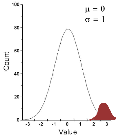
Population sampling from tail of distribution

Figure 1. Population sampling from tail of distribution

We would likely conclude that our sample mean is different (greater) than the population mean.

A type II error is committed, by chance alone, when our sample is between two different population distributions. The implication for our study is drawn in Figure 2. Instead of our sampling drawn from one population, we may have drawn between two very different populations.

Sample drawn between two populations

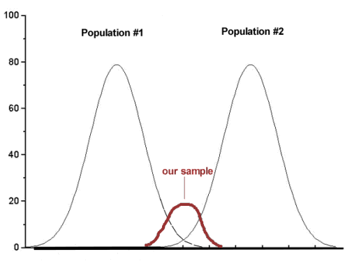
Figure 2. Without us knowing, our sample may come from the extremes of two separate populations.

How did we end up with “the wrong” sample? Recall from our first discussions about Experimental Design how we distinguished between random and haphazard sampling. The key concept was that a program of recruitment of subjects (e.g., how to get a sample) must be conducted in such a way that each member of the population has an equal chance of being included in the study. Only then can we be sure that extrinsic factors (things that influence our outcome but are not under our control nor do we study them) are spread over all groups, thus canceling out.

Why do we say we are 95% confident in our estimate (or conclusions)?

(1) Because we can never be 100% certain that by chance alone we haven’t gotten a biased sample (all it takes is a few subjects in some cases to “throw off” our results).

(2) For parametric tests, at least, we assume that we are sampling from a normal population.

Thus, in statistics, we need an additional concept. Not only do we need to know the probability of when we will be wrong (α, β), but we also want to know the probability of when we will be correct when we use a particular statistical test. This latter concept is defined as the power of a test as the probability of correctly rejecting Ho when it is false. Conducting a power analysis before starting the experiment can help answer basic experimental design questions like, how many subjects (experimental units) should my project include? What approximate differences, if any might I expect among the subjects? (Eng 2003; Cohen 1992)

Put another way, power is the likelihood of identifying a significant (important) effect (difference) when one exists. Formally, statistical power is defined as the probability, p = 1 – β, and it is the subject of this chapter.

Questions

True or False. If we reduce Type I error from 5% to 1%, our test of the null hypothesis has more power.
- Explain your selection to question 1.
True or False. Statistical power is linked to Type II error.
- Explain your selection to question 2.